Norman L. Biggs is a mathematician known for his work in the field of algebra and combinatorics. He has made significant contributions to various mathematical concepts and has authored several academic papers and books. One notable aspect of his work is related to group theory and its applications. If you are referring to something specific like a particular publication, theory, or topic associated with Norman L. Biggs, please provide more details for a more precise answer!
The rational normal curve is a mathematical concept often used in algebraic geometry and related fields. It is defined as the image of the embedding of projective space into a projective space of higher dimensions via a rational parameterization.
In combinatorial mathematics, a **necklace polynomial** is a polynomial that counts the number of different ways to color a necklace (or circular arrangement) made from beads of different colors, considering rotations as indistinguishable. The concept is a part of the field of combinatorial enumeration and is connected to group theory and Burnside's lemma.
Norman Macleod Ferrers (1829–1903) was a British mathematician known for his contributions to the field of mathematics, particularly in the areas of algebra and geometry. He is perhaps best recognized for his work relating to linear algebra and the study of algebraic forms and structures. Ferrers' work included the development of Ferrers diagrams, which are graphical representations used in combinatorics and the theory of partitions.
Nuclear technology in Sweden refers to the use of nuclear energy for electricity generation, research, and medical applications. Sweden has a well-established nuclear energy program that has been a significant part of the country's energy mix for decades. ### Key Aspects of Nuclear Technology in Sweden: 1. **Nuclear Power Plants**: Sweden has several operational nuclear power plants that generate a substantial portion of the country's electricity.
The term "opposite category" can be interpreted in various contexts depending on the field of study or discussion. Here are a few possible interpretations: 1. **Mathematics**: In category theory, a branch of mathematics, the opposite category (or dual category) of a category \( C \) is constructed by reversing the direction of all morphisms (arrows) in \( C \).
Opticians are professionals who specialize in eyewear and the fitting of lenses for vision correction. Their primary role involves interpreting prescriptions provided by optometrists or ophthalmologists and then designing, fitting, and dispensing eyeglasses and contact lenses. They may assist customers in selecting frames and lenses that suit their needs and preferences, taking into account factors like style, comfort, and optical requirements.
In mathematics, particularly in the study of complex analysis and singularity theory, an **ordinary singularity** refers to a type of singularity that appears in the context of complex functions or algebraic curves. More specifically, an ordinary singularity is often characterized by the behavior of the function or curve in the vicinity of the singular point.
Pakistani physicists are scientists from Pakistan who specialize in the field of physics. The country has produced a number of notable physicists who have made significant contributions to various areas of physics, such as theoretical physics, experimental physics, nuclear physics, astrophysics, and more.
Patrick Michael Grundy is a notable figure in the field of mathematics and computer science, particularly known for his contributions to graph theory, algorithm design, and optimization. He has engaged in various academic pursuits, including research and teaching. However, it's worth mentioning that his relevance may be specific to certain academic circles or developments within those fields, and information about him may vary.
Paul Churchland is a prominent Canadian philosopher and a leading figure in the philosophy of mind and cognitive science. He is best known for his work in naturalism, eliminative materialism, and the philosophy of neuroscience. Churchland argues against the idea of folk psychology—the everyday understanding of mental states such as beliefs and desires—and suggests that we should instead look to scientific accounts of the brain and mind.
The Paul F. Forman Team Engineering Excellence Award is presented by the Institute of Electrical and Electronics Engineers (IEEE) to recognize outstanding engineering teams that have made significant contributions to the field of electrical and electronics engineering. The award honors teams that demonstrate exceptional collaboration, creativity, and innovation in engineering projects, showcasing the impact of teamwork on achieving engineering excellence. The award is named after Paul F.
In electromagnetism, reciprocity refers to a principle that relates the response of a system to an electromagnetic field to the response of the same system when the source of the field and the observation point are interchanged. This principle is grounded in the linearity and time-invariance of many physical systems described by Maxwell's equations, which govern the behavior of electric and magnetic fields.
Pinned article: Introduction to the OurBigBook Project
Welcome to the OurBigBook Project! Our goal is to create the perfect publishing platform for STEM subjects, and get university-level students to write the best free STEM tutorials ever.
Everyone is welcome to create an account and play with the site: ourbigbook.com/go/register. We belive that students themselves can write amazing tutorials, but teachers are welcome too. You can write about anything you want, it doesn't have to be STEM or even educational. Silly test content is very welcome and you won't be penalized in any way. Just keep it legal!
Intro to OurBigBook
. Source. We have two killer features:
- topics: topics group articles by different users with the same title, e.g. here is the topic for the "Fundamental Theorem of Calculus" ourbigbook.com/go/topic/fundamental-theorem-of-calculusArticles of different users are sorted by upvote within each article page. This feature is a bit like:
- a Wikipedia where each user can have their own version of each article
- a Q&A website like Stack Overflow, where multiple people can give their views on a given topic, and the best ones are sorted by upvote. Except you don't need to wait for someone to ask first, and any topic goes, no matter how narrow or broad
This feature makes it possible for readers to find better explanations of any topic created by other writers. And it allows writers to create an explanation in a place that readers might actually find it.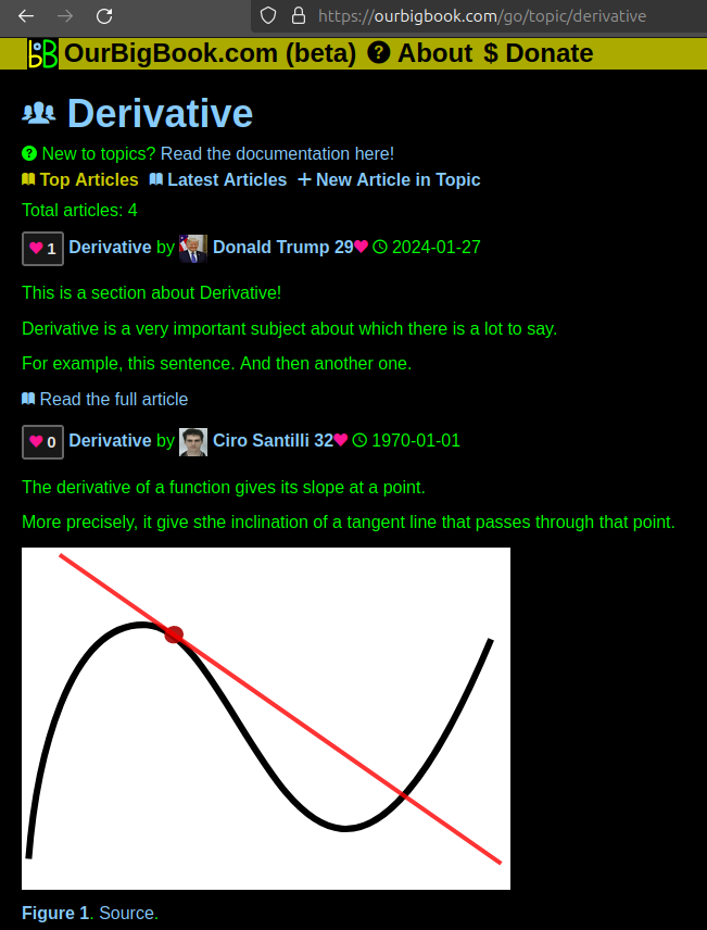
Figure 1. Screenshot of the "Derivative" topic page. View it live at: ourbigbook.com/go/topic/derivativeVideo 2. OurBigBook Web topics demo. Source. - local editing: you can store all your personal knowledge base content locally in a plaintext markup format that can be edited locally and published either:This way you can be sure that even if OurBigBook.com were to go down one day (which we have no plans to do as it is quite cheap to host!), your content will still be perfectly readable as a static site.
- to OurBigBook.com to get awesome multi-user features like topics and likes
- as HTML files to a static website, which you can host yourself for free on many external providers like GitHub Pages, and remain in full control

Figure 3. Visual Studio Code extension installation.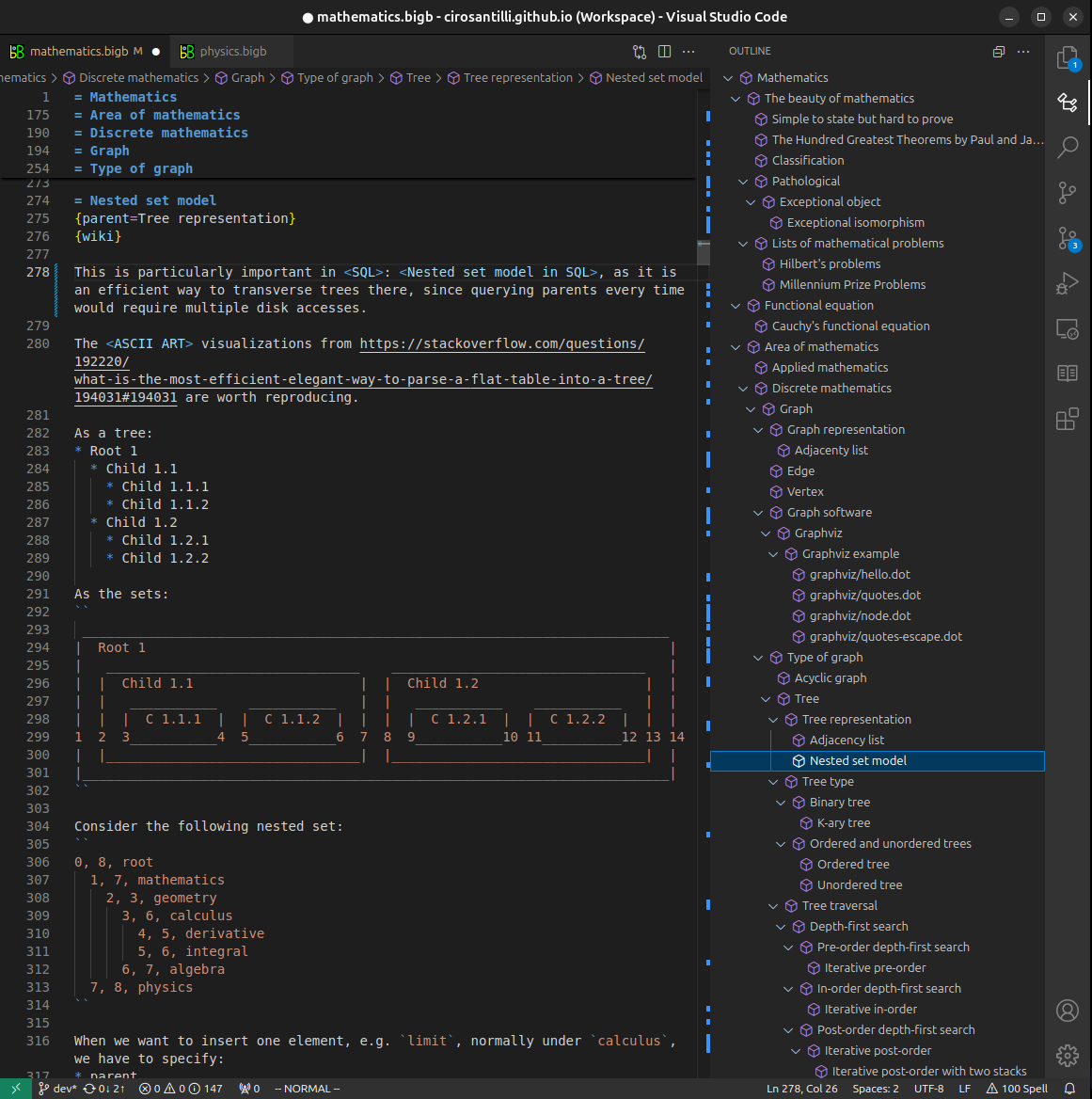
Figure 4. Visual Studio Code extension tree navigation.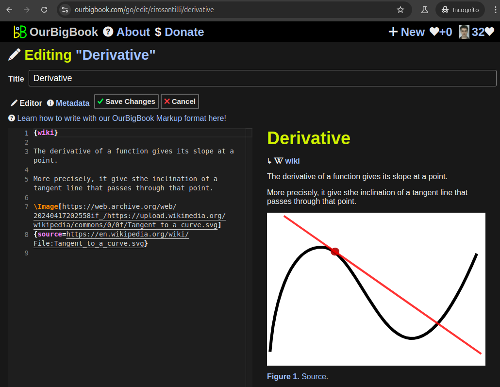
Figure 5. Web editor. You can also edit articles on the Web editor without installing anything locally.Video 3. Edit locally and publish demo. Source. This shows editing OurBigBook Markup and publishing it using the Visual Studio Code extension.Video 4. OurBigBook Visual Studio Code extension editing and navigation demo. Source. 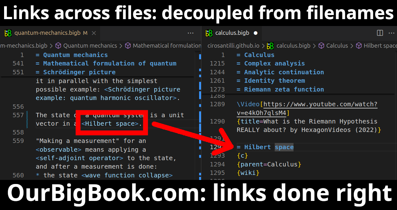
- Infinitely deep tables of contents:


All our software is open source and hosted at: github.com/ourbigbook/ourbigbook
Further documentation can be found at: docs.ourbigbook.com
Feel free to reach our to us for any help or suggestions: docs.ourbigbook.com/#contact