Sacred Harp refers to a tradition of shape-note singing that originated in the early 19th century in the United States, particularly in the southern states. The term "Sacred Harp" also specifically refers to a collection of hymns and songs that are written for this style of music. The Sacred Harp songbook, first published in 1844 and revised in subsequent years, features a variety of hymn writers and composers.
The Salvador Dalí House Museum, known as the "Casa Museo Salvador Dalí," is located in Port Lligat, Spain, near the town of Cadaqués on the Costa Brava. This museum was the home and studio of the surrealist artist Salvador Dalí, who lived there for much of his life with his wife, Gala. The house is notable not only as a residence but also as a reflection of Dalí's unique artistic vision.
Sandia National Laboratories is a multi-program laboratory managed and operated by the Sandia Corporation, a subsidiary of Lockheed Martin. Located primarily in Albuquerque, New Mexico, and Livermore, California, it is one of the U.S. Department of Energy's primary national laboratories. Sandia focuses on a wide range of research areas, including national security, energy, nuclear deterrence, and cybersecurity.
In physics, deflection refers to the displacement of a body or a beam from its original position under the influence of an external force. When an object is subjected to forces such as tension, compression, bending, or torsion, it can deform or bend, resulting in a change in its shape or position. Deflection is often measured as the distance that a point on the structure moves from its equilibrium position.
1:32 scale refers to a scale ratio commonly used in modeling and miniatures, where 1 unit of measurement on the model (e.g., an inch or a centimeter) represents 32 units of the same measurement in real life. This means that a model at 1:32 scale is 32 times smaller than the actual object it represents.
1:72 scale is a scale model ratio that indicates that one unit of measurement on the model represents 72 of the same units in reality. This means that an object modeled in this scale is 1/72nd the size of the actual object. For example, if a model airplane in 1:72 scale is 10 inches long, the real airplane would be 720 inches (or 60 feet) long.
Scattering, absorption, and radiative transfer are fundamental concepts in optics that describe how light interacts with matter. Here's a brief overview of each concept: ### Scattering Scattering refers to the deflection of light rays from a straight path due to interaction with particles or irregularities in a medium. When light encounters small particles (like dust, air molecules, or water droplets), it can be redirected in various directions.
Core-excited shape resonance is a phenomenon observed in the field of quantum mechanics and atomic physics, particularly in the context of electron scattering and the interaction of charged particles with matter. Here’s a summary of the key concepts involved: 1. **Shape Resonance**: This term generally refers to a type of resonance that occurs when an incoming particle experiences a potential barrier and the shape of the potential allows for the temporary trapping of the particle, leading to an enhancement of scattering processes.
Grazing-incidence small-angle scattering (GISAS) is a powerful experimental technique primarily used in materials science, physics, and biophysics to study thin films, nanostructures, and surfaces. It combines aspects of small-angle scattering (SAS) and grazing incidence techniques to provide valuable information about the structural properties of materials at the nanoscale.
Lattice scattering refers to the phenomenon where a particle, such as an electron or phonon, interacts with the regular periodic structure of a crystal lattice. This process is crucial in solid-state physics and materials science because it affects various properties of materials, including electrical conductivity, thermal conductivity, and the behavior of electrons in semiconductors. In more detail, in a crystalline solid, atoms are arranged in a repetitive pattern, forming a lattice.
Rosegarden is a music composition and editing software that is particularly popular among Linux users. It combines MIDI sequencing, digital audio recording, and score editing features, allowing musicians and composers to create, edit, and arrange music. Rosegarden provides a user-friendly interface for working with MIDI instruments and audio files, making it suitable for both amateur and professional musicians. Some key features of Rosegarden include: - MIDI sequencing: Users can create and manipulate MIDI tracks to compose music with virtual instruments or external MIDI hardware.
The Panama Civil Defense Seismic Network (Red Sismológica de la Defensa Civil de Panamá) is an initiative developed by Panama's civil defense authorities to monitor seismic activity in the region. The primary goal of this network is to provide real-time data and analyses regarding earthquakes and seismic events, which is vital for disaster preparedness and response efforts.
A neutron moisture gauge is an instrument used to measure the moisture content in soil, concrete, and other materials. It operates based on the principles of nuclear physics, specifically by utilizing low-energy neutrons to interact with hydrogen atoms found in water. ### How It Works: 1. **Source of Neutrons**: The gauge contains a radioactive source, typically americium-beryllium, that emits neutrons.
Turbidimetry is an analytical technique used to measure the cloudiness or turbidity of a liquid caused by the presence of suspended particles. It involves the assessment of how much light is scattered by particles in the solution when a beam of light passes through it. The more particles present, the higher the turbidity, which results in a greater scattering of light.
"Mathematicians by academic institution" typically refers to the classification or listing of mathematicians based on their affiliations with particular universities or research institutes. This can include well-known mathematicians who held positions at specific institutions, as well as current faculty members at universities renowned for their mathematics programs. For example, several prestigious academic institutions are known for their contributions to mathematics: 1. **Princeton University** - Home to many notable mathematicians, especially in fields like number theory and geometry.
Deluxe Music Construction Set is a music composition software that was popular in the late 1980s and early 1990s, particularly for the Commodore 64 and Amiga platforms. It allowed users to create and arrange music through a graphical user interface that featured a variety of tools for composing, editing, and mixing tracks.
Early Notation Typesetter (ENTS) is a concept that refers to a range of early technologies and methods used for typesetting printed materials. This includes the transition from manual typesetting with individual movable type letters to more advanced methods that eventually led to modern typesetting technologies.
The National Institute for Mathematical Sciences (NIMS) is a research institute in South Korea that focuses on various areas of mathematics and its applications. Established to promote mathematical research and collaboration, NIMS aims to contribute to both the theoretical development of mathematics and its practical application in fields such as science, engineering, and industry. The institute typically engages in activities such as conducting research, hosting seminars and workshops, and providing educational programs for students and researchers in mathematics.
Master Tracks Pro is a digital audio workstation (DAW) software designed for music composition, recording, and editing. It was developed to cater to musicians and producers looking for a versatile platform to create and produce music. Key features often associated with Master Tracks Pro include: 1. **MIDI and Audio Recording:** Users can record both MIDI and audio tracks, allowing for flexibility in music production.
Pinned article: Introduction to the OurBigBook Project
Welcome to the OurBigBook Project! Our goal is to create the perfect publishing platform for STEM subjects, and get university-level students to write the best free STEM tutorials ever.
Everyone is welcome to create an account and play with the site: ourbigbook.com/go/register. We belive that students themselves can write amazing tutorials, but teachers are welcome too. You can write about anything you want, it doesn't have to be STEM or even educational. Silly test content is very welcome and you won't be penalized in any way. Just keep it legal!
Intro to OurBigBook
. Source. We have two killer features:
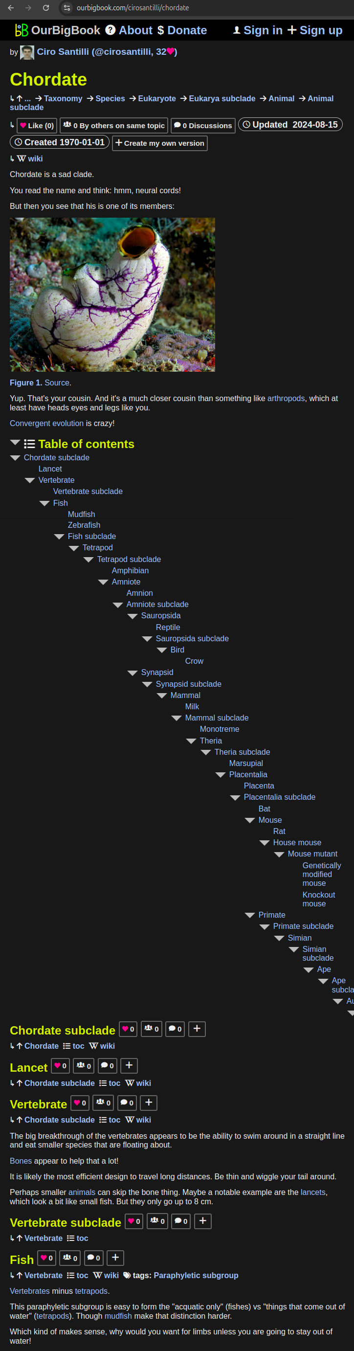
- topics: topics group articles by different users with the same title, e.g. here is the topic for the "Fundamental Theorem of Calculus" ourbigbook.com/go/topic/fundamental-theorem-of-calculusArticles of different users are sorted by upvote within each article page. This feature is a bit like:
- a Wikipedia where each user can have their own version of each article
- a Q&A website like Stack Overflow, where multiple people can give their views on a given topic, and the best ones are sorted by upvote. Except you don't need to wait for someone to ask first, and any topic goes, no matter how narrow or broad
This feature makes it possible for readers to find better explanations of any topic created by other writers. And it allows writers to create an explanation in a place that readers might actually find it.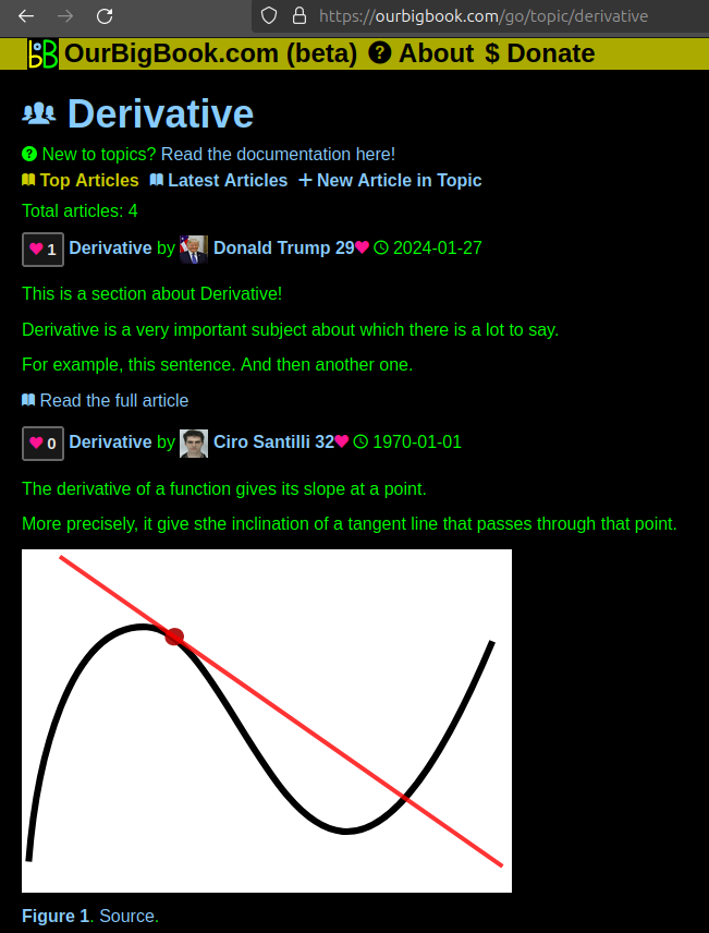
Figure 1. Screenshot of the "Derivative" topic page. View it live at: ourbigbook.com/go/topic/derivativeVideo 2. OurBigBook Web topics demo. Source. - local editing: you can store all your personal knowledge base content locally in a plaintext markup format that can be edited locally and published either:This way you can be sure that even if OurBigBook.com were to go down one day (which we have no plans to do as it is quite cheap to host!), your content will still be perfectly readable as a static site.
- to OurBigBook.com to get awesome multi-user features like topics and likes
- as HTML files to a static website, which you can host yourself for free on many external providers like GitHub Pages, and remain in full control
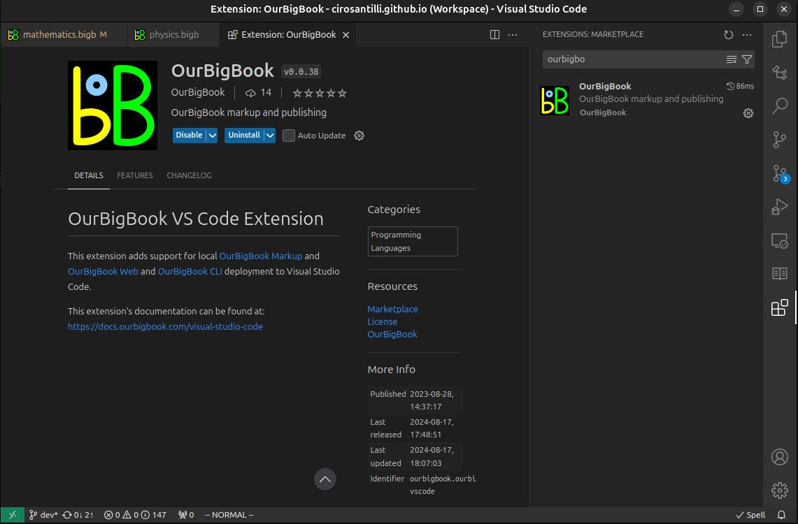
Figure 3. Visual Studio Code extension installation.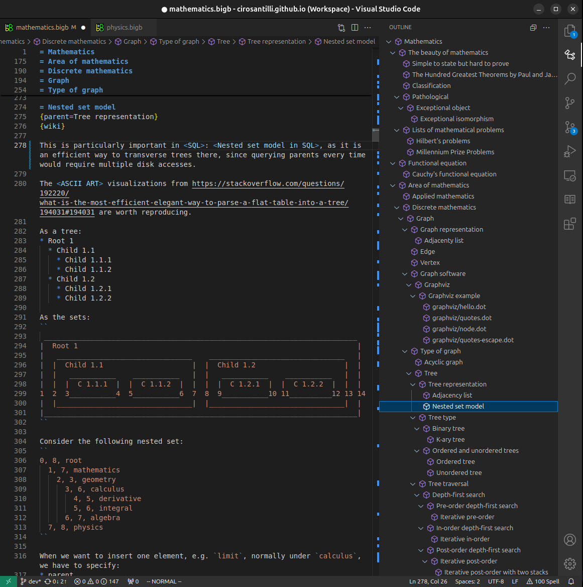
Figure 4. Visual Studio Code extension tree navigation.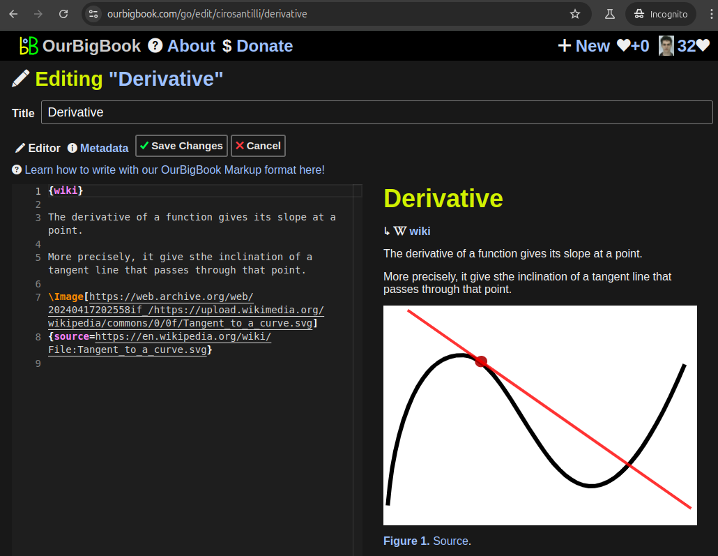
Figure 5. Web editor. You can also edit articles on the Web editor without installing anything locally.Video 3. Edit locally and publish demo. Source. This shows editing OurBigBook Markup and publishing it using the Visual Studio Code extension.Video 4. OurBigBook Visual Studio Code extension editing and navigation demo. Source. 
- Infinitely deep tables of contents:

All our software is open source and hosted at: github.com/ourbigbook/ourbigbook
Further documentation can be found at: docs.ourbigbook.com
Feel free to reach our to us for any help or suggestions: docs.ourbigbook.com/#contact