A **multipartite graph** is a specific type of graph used in graph theory, where the vertex set can be divided into multiple distinct subsets such that no two vertices within the same subset are adjacent. In other words, the edges of the graph only connect vertices from different subsets.
Chris Godsil is an American mathematician known for his work in the fields of algebra, combinatorics, and quantum computing. He is particularly recognized for his contributions to graph theory and representation theory. Godsil has authored or co-authored numerous papers and has also been involved in teaching and mentoring students in these areas of mathematics.
"Daniel Kráľ" could refer to a person, as it's a common name in some Slavic countries, particularly in Slovakia and the Czech Republic. However, without additional context, it is difficult to pinpoint exactly who or what you might be referring to. In general, "Daniel" is a common first name, and "Kráľ" translates to "king" in Slovak and Czech.
Frank Harary was an influential American mathematician known primarily for his contributions to the fields of graph theory and topology. He was born on May 8, 1921, and passed away on December 18, 2005. Harary is particularly well-known for introducing and popularizing various concepts in graph theory, including the study of networks and their applications.
Stirling numbers are a part of combinatorial mathematics and come in two main types: the Stirling numbers of the first kind and the Stirling numbers of the second kind. 1. **Stirling Numbers of the First Kind**: Denoted by \( c(n, k) \), these numbers count the number of permutations of \( n \) elements with exactly \( k \) disjoint cycles.
Giovanni Frattini may refer to a person, but there isn't a widely known figure by that name in public domains such as politics, arts, or sciences that stands out as of my last update in October 2023. It’s possible that he is a lesser-known individual or a private citizen. If you have more context, such as a specific field (e.g., sports, academia, etc.
Évariste Galois (1811–1832) was a French mathematician who made significant contributions to the field of abstract algebra. He is best known for developing what is now called Galois theory, which connects field theory and group theory in a profound way, providing a systematic way to study polynomial equations and their solutions. Galois's work primarily focused on understanding the solvability of polynomial equations in terms of group theory.
Symmetry in mechanics refers to properties or behaviors of mechanical systems that remain unchanged under certain transformations, such as translations, rotations, or reflections. Symmetry plays a fundamental role in understanding the physical behavior of systems, simplifying analyses, and identifying conserved quantities. Here are a few key aspects of symmetry in mechanics: 1. **Types of Symmetry**: - **Translational Symmetry**: A system exhibits translational symmetry if its properties are invariant under shifts in position.
Half-Life 2: Episode Three was meant to be the third installment in a series of episodic sequels to the critically acclaimed game Half-Life 2, developed by Valve Corporation. Announced alongside Half-Life 2: Episode One in 2006, Episode Three was intended to continue the story of protagonist Gordon Freeman and his struggle against the oppressive Combine forces, picking up where Episode Two left off.
A Hall-effect thruster (HET) is a type of electric propulsion system used primarily in spacecraft. It operates by utilizing the Hall effect to generate thrust through ionized propellant. Here is how it works: 1. **Ionization**: The thruster uses a noble gas, typically xenon, as propellant. Inside the thruster, this gas is ionized by an electric discharge, which turns it into plasma consisting of positively charged ions and free electrons.
The Quantum Hall transition refers to the phenomenon observed in two-dimensional electron systems subjected to strong magnetic fields at low temperatures, leading to quantized Hall conductance. This occurs when the system transitions between different quantum Hall states, characterized by distinct plateaus in the Hall conductance as the magnetic field is varied.
SMART-1, which stands for Small Missions for Advanced Research and Technology, was a European Space Agency (ESA) spacecraft that was launched on September 27, 2003. It was primarily designed as a technology demonstration mission to test various new technologies for future spacecraft.
The Liouville–Arnold theorem, also known as the Liouville–Arnold theorem of integrability, is a result in Hamiltonian mechanics concerning the integrability of Hamiltonian systems. It provides a criterion under which a dynamical system can be considered integrable in the sense of having as many conserved quantities as degrees of freedom, allowing the system to be solved in terms of action-angle variables.
The Weinstein conjecture is a hypothesis in the field of geometric topology and symplectic geometry, formulated by the mathematician Alan Weinstein in the 1970s. It concerns the existence of certain types of periodic orbits in Hamiltonian dynamical systems. More specifically, the conjecture posits that every closed, oriented, and compact contact manifold must contain at least one Reeb chord.
"Pintle" can refer to a couple of different concepts, primarily in engineering and maritime contexts: 1. **Pintle as a Mechanical Component**: In mechanical terms, a pintle is a type of bearing or pivot mechanism, typically a short shaft or pin that serves as a hinge or pivot point. Pintles are often used in conjunction with a socket or a similar component to allow for rotational movement. They are commonly found in applications such as steering systems, hinges, or rotating machinery.
The term "segmented spindle" typically refers to a type of mitotic spindle observed during cell division. In a standard mitotic process, the spindle apparatus, which is composed of microtubules, helps in the separation of chromosomes into daughter cells. A segmented spindle is characterized by a non-continuous arrangement of spindle fibers. This can happen in certain cells or under specific conditions, often observed in some types of cancerous cells or during particular stages of cell division.

Prototype: github.com/cirosantilli/Urho3D-cheat
Top Down 2D Continuous Game with Urho3D C++ SDL and Box2D for Reinforcement learning by Ciro Santilli (2018)
Source. Source code at: github.com/cirosantilli/Urho3D-cheat.
Screenshot of the basketball stage of Ciro's 2D continuous game
. Source code at: github.com/cirosantilli/rl-game-2d-grid. Big kudos to game-icons.net for the sprites.Less good discrete prototype: github.com/cirosantilli/rl-game-2d-grid YouTube demo: Video 1. "Top Down 2D Continuous Game with Urho3D C++ SDL and Box2D for Reinforcement learning by Ciro Santilli (2018)".
Top Down 2D Discrete Tile Based Game with C++ SDL and Boost R-Tree for Reinforcement Learning by Ciro Santilli (2017)
Source. The goal of this project is to reach artificial general intelligence.
A few initiatives have created reasonable sets of robotics-like games for the purposes of AI development, most notably: OpenAI and DeepMind.
However, all projects so far have only created sets of unrelated games, or worse: focused on closed games designed for humans!
What is really needed is to create a single cohesive game world, designed specifically for this purpose, and with a very large number of game mechanics.
Notably, by "game mechanic" is meant "a magic aspect of the game world, which cannot be explained by object's location and inertia alone" in order to test the the missing link between continuous and discrete AI.
The question then becomes: do we have enough computational power to simulation a game worlds that is analogous enough to the real world, so that our AI algorithms will also apply to the real world?
To reduce computation requirements, it is better to focus on a 2D world at first. Such world with the right mechanics can break any AI, while still being faster to simulate than a 3D world.
The initial prototype uses the Urho3D open source game engine, and that is a reasonable project, but a raw Simple DirectMedia Layer + Box2D + OpenGL solution from scratch would be faster to develop for this use case, since Urho3D has a lot of human-gaming features that are not needed, and because 2019 Urho3D lead developers disagree with the China censored keyword attack.
Simulations such as these can be viewed as a form of synthetic data generation procedure, where the goal is to use computer worlds to reduce the costs of experiments and to improve reproducibility.
Ciro has always had a feeling that AI research in the 2020's is too unambitious. How many teams are actually aiming for AGI? When he then read Superintelligence by Nick Bostrom (2014) it said the same. AGI research has become a taboo in the early 21st century.
Related projects:
- github.com/deepmind/lab2d: 2D gridworld games, C++ with Lua bindings
Related ideas:
- www.youtube.com/watch?v=MHFrhIAj0ME?t=4183 Can't get you out of my head by Adam Curtis (2021) Part 1: Bloodshed on Wolf Mountain :)
- www.youtube.com/watch?v=EUjc1WuyPT8 AI alignment: Why It's Hard, and Where to Start by Eliezer Yudkowsky (2016)
Bibliograpy:
- agents.inf.ed.ac.uk/blog/multiagent-learning-environments/ Multi-Agent Learning Environments (2021) by Lukas Schäfer from the Autonomous agents research group of the University of Edinburgh. One of their games actually uses apples as visual represntation of rewards, exactly like Ciro's game. So funny. They also have a 2d continuous game: agents.inf.ed.ac.uk/blog/multiagent-learning-environments/#mpe
- humanoid robot simulation
- Section "AI training game"
- Section "Software-based artificial life"
Much bigger simulation, AIs learn Phalanx by Pezzza's Work (2022)
Source. 2d agents with vision. Simple prey/predator scenario.Kaʻula is a small, uninhabited island located in the Hawaiian Archipelago, specifically situated about 18 miles (29 kilometers) west of the island of Kauai. It is part of the Northwestern Hawaiian Islands and is known for its rugged terrain and diverse ecosystems. Kaʻula was formed through volcanic activity, and its geography includes steep cliffs, rocky shores, and some vegetation.
Laser Flash Analysis (LFA) is a technique used primarily to measure the thermal conductivity of materials. It involves heating a sample using a short laser pulse and then measuring the temperature rise on the opposite side of the sample over time. The key components of the LFA method include: 1. **Sample Preparation**: The material being tested is typically in the form of a thin disc or pellet, which should be uniform in thickness and density.
Pinned article: Introduction to the OurBigBook Project
Welcome to the OurBigBook Project! Our goal is to create the perfect publishing platform for STEM subjects, and get university-level students to write the best free STEM tutorials ever.
Everyone is welcome to create an account and play with the site: ourbigbook.com/go/register. We belive that students themselves can write amazing tutorials, but teachers are welcome too. You can write about anything you want, it doesn't have to be STEM or even educational. Silly test content is very welcome and you won't be penalized in any way. Just keep it legal!
Intro to OurBigBook
. Source. We have two killer features:
- topics: topics group articles by different users with the same title, e.g. here is the topic for the "Fundamental Theorem of Calculus" ourbigbook.com/go/topic/fundamental-theorem-of-calculusArticles of different users are sorted by upvote within each article page. This feature is a bit like:
- a Wikipedia where each user can have their own version of each article
- a Q&A website like Stack Overflow, where multiple people can give their views on a given topic, and the best ones are sorted by upvote. Except you don't need to wait for someone to ask first, and any topic goes, no matter how narrow or broad
This feature makes it possible for readers to find better explanations of any topic created by other writers. And it allows writers to create an explanation in a place that readers might actually find it.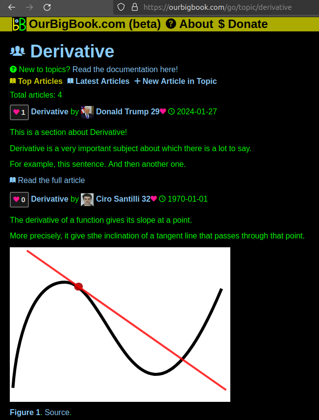
Figure 1. Screenshot of the "Derivative" topic page. View it live at: ourbigbook.com/go/topic/derivativeVideo 2. OurBigBook Web topics demo. Source. - local editing: you can store all your personal knowledge base content locally in a plaintext markup format that can be edited locally and published either:This way you can be sure that even if OurBigBook.com were to go down one day (which we have no plans to do as it is quite cheap to host!), your content will still be perfectly readable as a static site.
- to OurBigBook.com to get awesome multi-user features like topics and likes
- as HTML files to a static website, which you can host yourself for free on many external providers like GitHub Pages, and remain in full control

Figure 3. Visual Studio Code extension installation.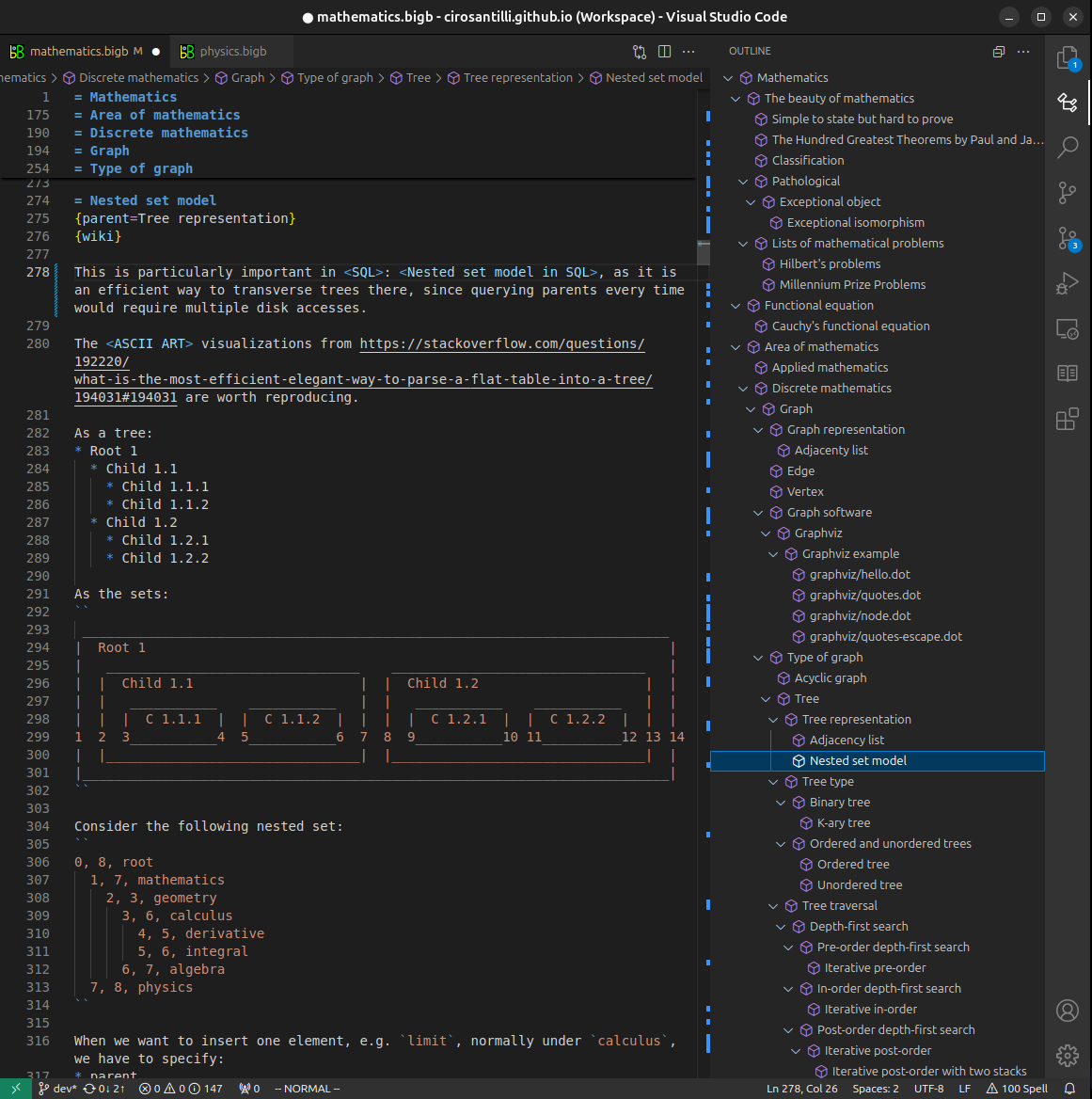
Figure 4. Visual Studio Code extension tree navigation.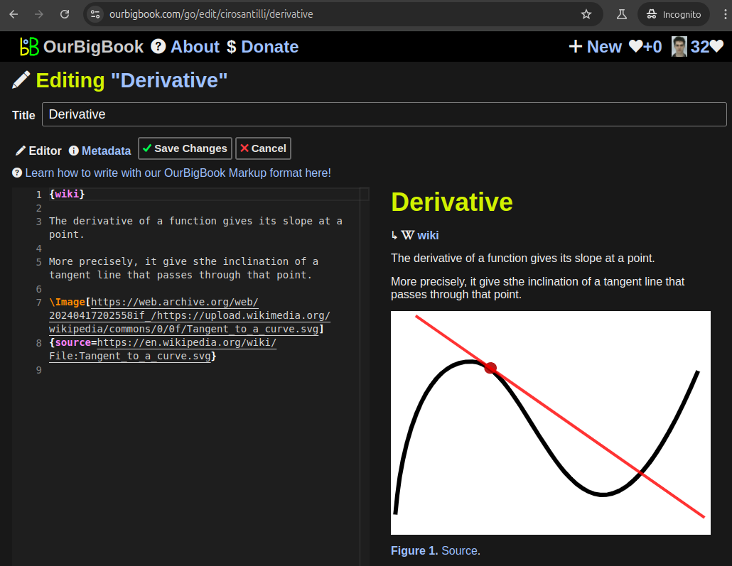
Figure 5. Web editor. You can also edit articles on the Web editor without installing anything locally.Video 3. Edit locally and publish demo. Source. This shows editing OurBigBook Markup and publishing it using the Visual Studio Code extension.Video 4. OurBigBook Visual Studio Code extension editing and navigation demo. Source. 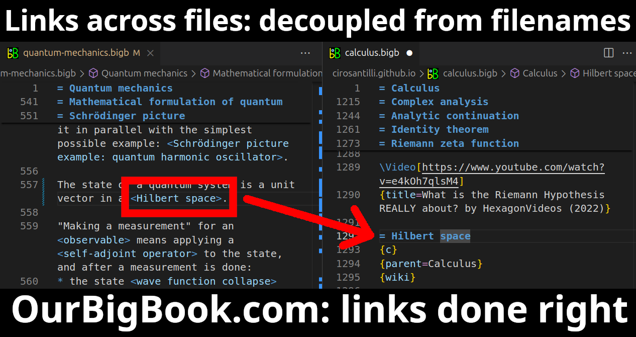
- Infinitely deep tables of contents:

All our software is open source and hosted at: github.com/ourbigbook/ourbigbook
Further documentation can be found at: docs.ourbigbook.com
Feel free to reach our to us for any help or suggestions: docs.ourbigbook.com/#contact