Law of total probability

Let $(B_i)$ be a countable measurable partition of the sample space, with positive probabilities. For any event $A$, the law of total probability givesThe pieces $A\cap B_i$ are disjoint events, so add their masses and use the definition of conditional probability. Zero-mass partition pieces can be omitted without changing the answer.

For the coin selection in probability, let $B$ mean the $3/4$-head coin was selected and let $H$ mean the first toss was heads. Then $\mathbb{P}(H)=\mathbb{P}(H\mid B)\mathbb{P}(B)+\mathbb{P}(H\mid B^c)\mathbb{P}(B^c)=11/20$. Each conditional answer describes one possible hidden situation; its weight describes how often that situation occurs under the model. This decomposition is useful whenever a simple conditional model sits behind a more complicated marginal probability distribution.

The law of total probability combines local conditional probabilities into one overall probability. The measurable partition must cover the sample space with pairwise disjoint events: every elementary outcome belongs to exactly one part. Its probabilities are the weights of a weighted mean, and they sum to one.^[ref]

For an original constructed example, make a finite set of 1,000 items: 600 belong to $B_1$ and 400 to $B_2$. Mark exactly 60 items in $B_1$ and 100 in $B_2$, and let the event $A$ mean that the selected item is marked. Select an item using the uniform distribution on a finite set. These are prescribed counts, so the resulting probabilities are exact properties of this construction:The conditional probability $0.1$ uses only the 600 items in $B_1$ as its denominator. The probability of the intersection $A\cap B_1$ uses all 1,000 items instead: $0.6\times 0.1=0.06$. Similarly, $\mathbb{P}(A\cap B_2)=0.4\times 0.25=0.10$. Adding the two disjoint events gives

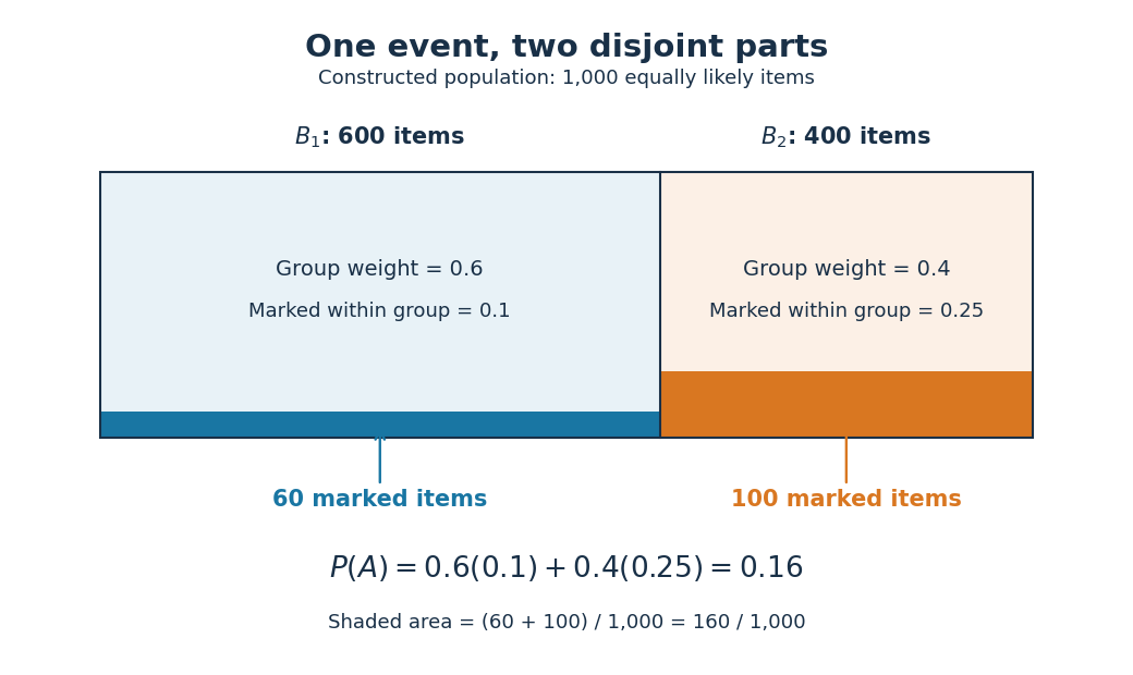
An unweighted arithmetic mean of the two conditional probabilities would give $(0.1+0.25)/2=0.175$. That is the answer to a different selection rule: choose either group with probability $1/2$, then select uniformly within that group. Here the first group contains more items, so selecting uniformly among all items gives it weight $0.6$. In fact, if its weight were $w$, the overall probability would be $0.1w+0.25(1-w)=0.25-0.15w$. Moving the weight from $1/2$ to $0.6$ lowers the result by $0.015$, explaining exactly why $0.175$ is too large for the original model.

The same construction is a mixture distribution: first select a group with its mixture weight, then select an item within that group. Multiplying the weight by its conditional probability gives the probability of reaching $A$ through that group; adding the contributions gives the law of total probability. For example, an item in $B_1$ has selection probability $0.6/600=1/1000$, and an item in $B_2$ has selection probability $0.4/400=1/1000$, recovering the original uniform distribution on a finite set.

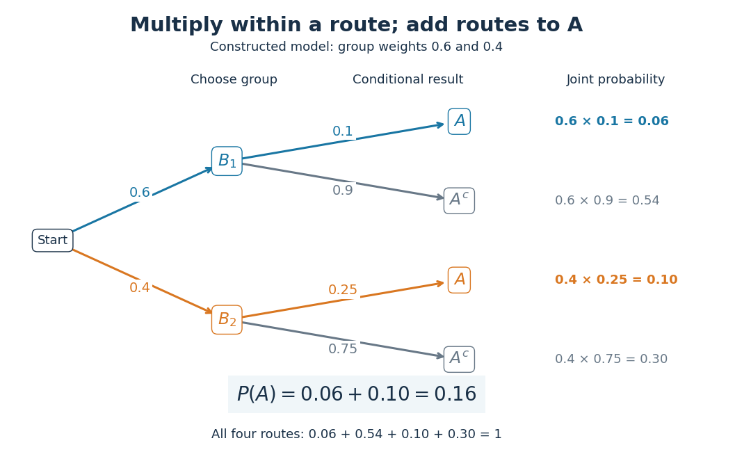
No assumption of independent events is needed. In this construction $\mathbb{P}(A\mid B_1)=0.1$ differs from $\mathbb{P}(A)=0.16$, so $A$ and $B_1$ are not independent events. Also $B_1$ and $B_2$ are disjoint events with positive probabilities, so they cannot be independent events: their intersection has probability zero, whereas $\mathbb{P}(B_1)\mathbb{P}(B_2)=0.24$. The measurable partition supplies exclusive alternatives, not an independence assumption.

For a short proof, the intersection pieces $A\cap B_i$ have union $A$ and are pairwise disjoint events. Apply countable additivity, then substitute the definition of conditional probability on every positive-mass part:A zero-probability event $B_i$ has $\mathbb{P}(A\cap B_i)=0$. Omit it: writing $\mathbb{P}(A\mid B_i)$ would divide by zero. Countability ensures that the union of the omitted zero-probability events also has probability zero. Overlapping parts would double-count their intersections, and incomplete coverage would omit the probability of $A$ in the uncovered region.^[ref]

Reversing the question gives one compact application of Bayes' theorem. Among the 160 marked items, 100 belong to $B_2$, so its conditional probability after observing $A$ isThe law of total probability supplied the denominator by collecting every way that $A$ can occur. Its usefulness lies in choosing a measurable partition where the conditional probabilities are simple, then combining them without losing the relative sizes of the alternatives.