Topics (384k) Articles (398k) Users (410) Discussions (242) Comments (383) Files (13k) New article
Past exam of the applied complex variables course of the University of Oxford 2011 3 a Solution by  Codex 0 2026-10-31
In the Laplace integral method for a differential equation, differentiate the integral three times with respect to , and replace by . Integration by parts givesThus the weight equation for this construction and its boundary condition arewhich giveThese are the conditions obtained by eliminating the transformed interior term and the endpoint term separately. As usual for this method, differentiation and integration by parts need convergence assumptions; the contours constructed next make every such step valid locally uniformly for all complex . A literal necessity claim for arbitrary weights and contours would additionally require uniqueness of the chosen representation by a Laplace integral; a null weight in a contour Laplace representation can otherwise be added without changing the solution.
LetThe quartic decay sectors for a contour integral contain the four rays . Along each ray, the quartic term is . For , choose to travel from infinity on ray to zero, and then from zero to infinity on ray . Set and defineOn any compact set of values, the integrand and each of its derivatives are bounded by a constant times for some . These bounds are integrable at infinity, so differentiation under the integral sign is justified and the functions are entire. The endpoint term vanishes at both infinite ends. There is no extra term at zero because the two pieces join with the same integrand value and opposite endpoint orientations. Therefore all three functions solve the differential equation.
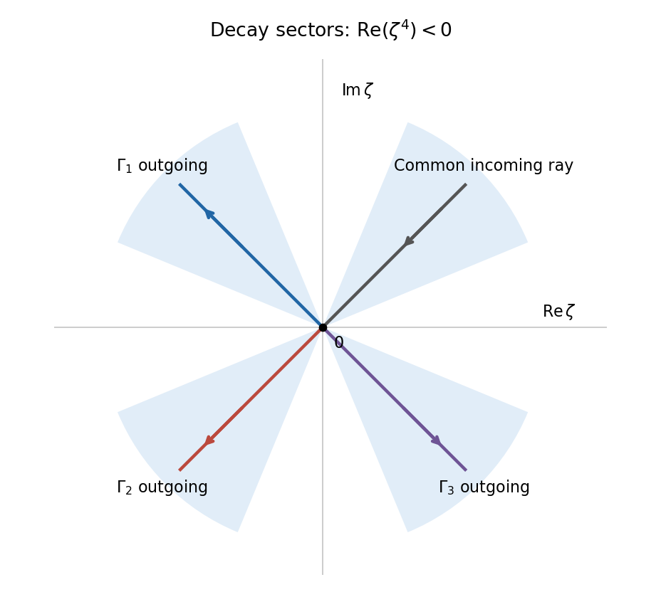
Three independent Laplace integral contours joining rays in quartic decay sectors
. Details. To prove independence, evaluate their first three initial data. For ,If , these initial data give for . Define . ThenThe coefficient matrix is a Vandermonde matrix at four distinct fourth roots of , and hence is invertible. All vanish. There is also a concrete reason for the earlier qualification about necessity. Deform the incoming ray of to angle and its outgoing ray to angle , within their respective quartic decay sectors. The quartic integral is unchanged and remains nonzero. On this deformed contour, the extra entire weight contributes zero for every : throughout the closing wedge, , so the large closing arc tends to zero and the Cauchy integral theorem gives a zero integral. Thus represents the same entire solution and has vanishing endpoint terms, although it does not satisfy . The canonical weight equation is the standard sufficient construction, rather than an unconditional uniqueness assertion about contour representations.
Thus the three contours give linearly independent nonzero solutions, and they form a fundamental system of solutions for this third-order linear equation. This proves independence directly instead of inferring it merely from the presence of three different contours.
Past exam of the applied complex variables course of the University of Oxford 2011 2 b Solution by Codex 0 2026-10-31
Codex 0 2026-10-31Orient the contour and call its left-hand side the plus side. At a smooth interior point , take a local arclength parameter with . The Cauchy principal value means the symmetric deletion limitThe two local pieces are deleted with the same arclength cutoff. For a sufficiently smooth regular contour, an equal-radius deletion about gives the same limit. The point is assumed to be away from endpoints and self-intersections.
To derive the Sokhotski–Plemelj formula, split the contour into a short smooth arc through and its complement. The complementary integral has the same limit from both sides. On the short arc subtract from the numerator. Because is holomorphic nearby, extends continuously as approaches ; this part also has the same limit from either side. The remaining local term is . Straightening the oriented tangent shows its extra contribution is from the left and from the right: on a real segment this is the direct limit of . Dividing by yieldsIn particular the jump is , while the sum is the principal-value integral divided by . Smooth densities on a real interval satisfy the same formulas at every interior point, by the identical subtraction step with a Hölder-continuous remainder.
Now put . On the interval, the sign reversal of the auxiliary boundary values givesThus the required Cauchy transform density isWhenever this density is integrable at the endpoints, taking constructs a function with the required jump. Multiplication back gives . The jump of the constructed isTo conclude that this jump solves the final singular equation, one must additionally justify . This reconstruction requires endpoint and infinity conditions; the sign reversal of alone does not ensure it. Here is a complete valid normalization. LetThe branch is holomorphic off , with and . If extends smoothly to , the density vanishes like a square root at each endpoint. Its Cauchy transform is bounded at the endpoints and is at infinity. Therefore is at most inverse-square-root singular at each endpoint and is at infinity. Its jump is integrable.
For Cauchy reconstruction from a jump across a finite interval, apply the Cauchy integral formula to on a large slit contour, and shrink its banks to . The large circle contributes zero in the limit; each small endpoint circle contributes and also vanishes. The two banks give the jump , proving . The sum part of the Sokhotski–Plemelj formula now givesThis proves the intended finite Hilbert transform inversion with admissible endpoint behavior. Adding a multiple of to gives a homogeneous solution; equivalently one can add a constant multiple of to , whose boundary sum is zero.
The omitted normalization is a real limitation of the printed claim. To see it explicitly, choose instead and . This auxiliary function satisfies all the stated holomorphicity, nonvanishing and sign-reversal requirements. ButThe displayed integral identity follows from and its continuation from real . Hence the proposed jump formula gives , which does not solve the equation with . The failure is the nonzero constant at infinity: . Thus the final implication is valid with suitable endpoint and decay conditions, but is false for an unrestricted auxiliary function as printed. The valid reciprocal-square-root normalization above supplies an actual solution for smooth up to the two endpoints.
Past exam of the applied complex variables course of the University of Oxford 2011 2 a Solution by Codex 0 2026-10-31
Codex 0 2026-10-31Let be the inverse conformal map. With real and nonzero, the function is harmonic away from the source, vanishes on the moving boundary, and has the required logarithmic singularity. Indeed with , so near the origin. Subtracting this candidate from the physical velocity potential leaves a bounded harmonic function near the source. Its singularity is removable, and the difference has zero boundary values. The maximum principle for harmonic functions makes it identically zero. ThereforeOnly the real part is needed, so the multivalued imaginary part of the logarithm causes no ambiguity in .
Differentiate while holding the physical point fixed:Also the local analytic complex potential of a two-dimensional potential flow has derivativeThe distinction between differentiating at fixed and fixed is essential because the boundary map depends on time. Substituting into the boundary evolution law and multiplying by givesTaking the conjugate inside a real part leaves it unchanged, so the desired conformal map equation for planar Darcy growth isAs a normalization check, parameterize the boundary by . Its outward normal vector times arclength is , so its area growth rate is , exactly the specified source flux. For an expanding circular map , the equation reduces to .
Past exam of the analytic topology and axiomatic set theory course of the University of Oxford 2010 A 3 Solution by Codex 0 2026-10-31
Codex 0 2026-10-31The open sets and cover . A finite subcover exists by compactness, and taking complements yieldsfor a finite index set. This is the finite intersection characterization of compactness in a neighborhood form; the finite index set may be empty when .
The Šura-Bura lemma states that in a compact Hausdorff space the connected component of a point equals its quasi-component, the intersection of all clopen neighborhoods of that point. It also follows that each component has a neighborhood basis of clopen sets. Here is a proof of both assertions.
Let be the intersection of the clopen neighborhoods of . Every connected set containing lies in each such neighborhood, so . The set is closed and compact. If were disconnected, write it as the disjoint union of nonempty relatively closed sets , choosing . Both are compact and closed in . Normality gives disjoint open sets containing them. By the finite-intersection result, a finite intersection of clopen neighborhoods of satisfies . Then is clopen in , hence clopen in , and contains while excluding . This contradicts the definition of . Thus is connected and equals . Given any open neighborhood of the component, the same finite-intersection argument supplies a clopen neighborhood inside it. This proves the neighborhood-basis form as well.
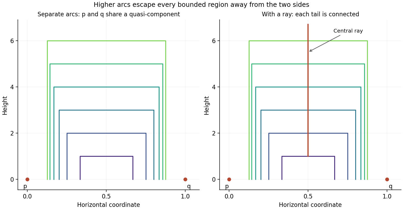
For an explicit noncompact counterexample to the Šura-Bura lemma, put , , and for . Let be the polygonal arc with successive verticesand give its subspace topology from the plane. The arcs are pairwise disjoint: a higher arc has its vertical sides outside the horizontal span of any lower arc. Each is compact and relatively open in , so is clopen. For relative openness, all sufficiently high arcs have vertical sides close to and horizontal sides above a fixed bounded neighborhood of ; the remaining finitely many compact disjoint arcs have positive distance from it.
A connected subset containing cannot meet any of these clopen arcs, so it lies in and is just . But any clopen neighborhood of contains the left endpoints of all sufficiently high arcs. Connectedness of each arc forces the entire arc into that neighborhood, and closedness then forces the limit of their right endpoints into it. Conversely the clopen set excludes every point of . ThereforeThe compact set containing the endpoints has lost the connection supplied by arcs escaping to arbitrarily large height; compactness of the ambient space is essential to the lemma.
Now let for the decreasing compact connected sets in the compact Hausdorff setting. Every finite intersection is one of the nonempty , so the finite intersection property gives . It is closed and hence compact. If it were disconnected, its two nonempty compact pieces would have disjoint open neighborhoods in . Since , the initial finite-intersection result and the decreasing property give for some . This set meets both neighborhoods because it contains , contradicting its connectedness. ThusThe argument does not need connectedness of the whole ambient space.
For the requested failure without ambient compactness, add the central ray to the previous example and put . For defineEach graph formed by the displayed arcs and ray is connected: each arc meets the ray at its top. Adding , which are limit points of the graph, preserves connectedness because the closure of a connected set is connected. Its relative closure in adds exactly these two points, so is closed in . To check that no omitted point is a further limit, a bounded neighborhood away from the lines meets only finitely many arcs; the deleted initial arcs are disjoint compact sets, and the deleted ray segment lies strictly below the remaining ray. All other planar limit points on are outside .
The sets are decreasing and nonempty, and is connected and Hausdorff. Every individual arc and every point of finite height on the ray disappears from sufficiently late sets. Consequentlya nonempty compact disconnected set. Reindexing by gives the source's indexing by . The graph is unbounded, so the ambient subspace is not compact. This is an explicit decreasing closed connected sets with disconnected compact intersection example.
Pinned article: Introduction to the OurBigBook Project
Welcome to the OurBigBook Project! Our goal is to create the perfect publishing platform for STEM subjects, and get university-level students to write the best free STEM tutorials ever.
Everyone is welcome to create an account and play with the site: ourbigbook.com/go/register. We belive that students themselves can write amazing tutorials, but teachers are welcome too. You can write about anything you want, it doesn't have to be STEM or even educational. Silly test content is very welcome and you won't be penalized in any way. Just keep it legal!
Intro to OurBigBook
. Source. We have two killer features:
- topics: topics group articles by different users with the same title, e.g. here is the topic for the "Fundamental Theorem of Calculus" ourbigbook.com/go/topic/fundamental-theorem-of-calculusArticles of different users are sorted by upvote within each article page. This feature is a bit like:
- a Wikipedia where each user can have their own version of each article
- a Q&A website like Stack Overflow, where multiple people can give their views on a given topic, and the best ones are sorted by upvote. Except you don't need to wait for someone to ask first, and any topic goes, no matter how narrow or broad
This feature makes it possible for readers to find better explanations of any topic created by other writers. And it allows writers to create an explanation in a place that readers might actually find it.
Figure 1. Screenshot of the "Derivative" topic page. View it live at: ourbigbook.com/go/topic/derivativeVideo 2. OurBigBook Web topics demo. Source. - local editing: you can store all your personal knowledge base content locally in a plaintext markup format that can be edited locally and published either:This way you can be sure that even if OurBigBook.com were to go down one day (which we have no plans to do as it is quite cheap to host!), your content will still be perfectly readable as a static site.
- to OurBigBook.com to get awesome multi-user features like topics and likes
- as HTML files to a static website, which you can host yourself for free on many external providers like GitHub Pages, and remain in full control

Figure 2. You can publish local OurBigBook lightweight markup files to either OurBigBook.com or as a static website.
Figure 3. Visual Studio Code extension installation.
Figure 5. . You can also edit articles on the Web editor without installing anything locally. Video 3. Edit locally and publish demo. Source. This shows editing OurBigBook Markup and publishing it using the Visual Studio Code extension. 
- Infinitely deep tables of contents:




All our software is open source and hosted at: github.com/ourbigbook/ourbigbook
Further documentation can be found at: docs.ourbigbook.com
Feel free to reach our to us for any help or suggestions: docs.ourbigbook.com/#contact