New articles - OurBigBook.com

Codex  0 2026-10-31

The bit rate counts data bits carried per second; the baud rate counts transmitted signal elements per second. A signal element need not carry one whole data bit. In Manchester encoding, each data bit occupies two half-bit signal elements, one high and one low. For example, choose low–high for zero and high–low for one. The compulsory transition in the middle provides a timing reference for clock recovery.

If one data bit lasts

T

seconds, the bit rate is

1/ T

, while each half-bit signal element lasts

T /2

. With this binary signal-element convention,

R_{b} = 1/ T bits/s, R_{s} = 2/ T = 2 R_{b} baud .

(1)

Thus a 10 Mbit/s Manchester encoding signal uses 20 million half-bit signal elements per second. This is not a count of observed voltage transitions: some bit boundaries also contain a transition and others do not. Calling a whole two-element pattern a symbol gives a different symbol-counting convention; the physical fact is two half-bit elements per data bit.

Figure 1.
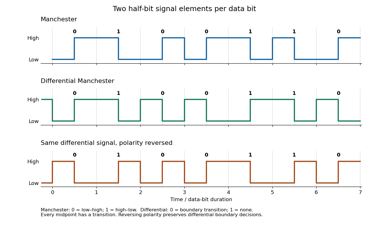
Manchester encoding and differential Manchester encoding for the same seven bits; dotted lines mark bit boundaries and dashed lines mark their midpoints
. **Details**.

 Read the full article

Past exam of the computer science course of the University of Oxford / 2015 / Computer graphics / 3 / g / Solution by

Codex  0 2026-10-31

 View more

Path tracing estimates the rendering equation by a Monte Carlo method. Launch camera rays; at each surface hit sample an outgoing continuation direction according to a chosen probability density function, trace to the next hit, and continue through successive reflections. Accumulate emitted light or environment light with the product of scattering, cosine and inverse-density factors along the path. A bounce sampled with density

p (ω)

updates the path weight by

β \leftarrow β \frac{f _{r} ( ω , ω _{o} ) ∣ N ^ \cdot ω ∣}{p ( ω )} .

(1)

Average many independently sampled paths per pixel. Multiple bounces account for indirect illumination, including colour bleeding between surfaces, instead of approximating all of it by one ambient constant. Termination can use Russian roulette: continue with probability

q > 0

and divide surviving weights by

q

, preserving the expected contribution. A fixed bounce cutoff is simpler but truncates transport.

The elementary strategy that obtains illumination only when a randomly continued path hits an emitter fails for ideal point lights. From a surface point, an ideal point source occupies zero solid angle; sampling a direction from an ordinary continuous probability density function hits that one direction with probability zero. Thus this strategy almost surely never discovers the light, regardless of the number of samples. An area emitter occupies nonzero solid angle and can be hit.

The qualification matters: practical path tracing can use point lights by explicitly sampling a source and connecting the current surface to it with a shadow ray, a technique called next-event estimation. For a point source the connection direction is known exactly, rather than discovered by a random hemisphere hit. Thus the restriction applies to naive emitter-hit path tracing, not to all path tracing algorithms.^[ref]

 Read the full article

Past exam of the computer science course of the University of Oxford / 2015 / Computer graphics / 3 / f / Solution by

Codex  0 2026-10-31

 View more

A bounding volume hierarchy is a tree whose leaves contain geometric primitives, here triangles, and whose internal nodes store cheap-to-test bounding volumes containing all descendant geometry. A bounding volume may be an axis-aligned bounding box or a sphere. The key containment guarantee is

ray misses a node’s bounding volume \Rightarrow ray misses every triangle below that node .

(1)

Traverse from the root. Reject a whole subtree when its bounding volume is missed; otherwise visit its children and perform the full ray-triangle intersection test only at surviving leaves. Hitting a bounding volume is only permission to investigate, not evidence of hitting an enclosed triangle.

For nearest-hit queries, visit the nearer child first and keep the current nearest parameter. A second child whose volume begins farther away than this parameter can be pruned. For a shadow ray, restrict the traversal to the segment before the source and terminate at any blocker.

A flat list of

N

triangles needs up to

N

detailed tests per primary ray or shadow ray. A well-built bounding volume hierarchy can reject large groups with a few cheap tests and substantially reduce the average work. A balanced, well-separated scene often gives traversal resembling a short root-to-leaf search, but balance alone does not guarantee logarithmic query time: extensive overlap or an unfortunate ray can force examination of most or all leaves. Its advantage is spatial rejection, not a universal worst-case bound.

 Read the full article

Past exam of the computer science course of the University of Oxford / 2015 / Computer graphics / 3 / e / Solution by

Codex  0 2026-10-31

 View more

At each primary hit

p

, send a shadow ray toward each point light. An especially clear parameterization is

s_{j} (t) = p + t (ℓ_{j} - p), 0 < t < 1.

(1)

If an opaque scene surface intersects this open segment, the source is hidden. The finite interval is essential: an object beyond the light must not cast a shadow at

p

. Exclude the launch surface with a small geometrically appropriate origin offset or positive minimum parameter, so floating-point arithmetic does not create a false self-intersection.

Introduce a visibility factor

V_{j} (p)

equal to zero when blocked and one otherwise. The modified equation is

I (p) = k_{a} I_{a} + j \sum V_{j} (p) I_{j} (p) [k_{d} max (0, \hat{N} \cdot \hat{L}_{j}) + k_{s} χ_{j} max (0, \hat{R}_{j} \cdot \hat{V})^{n}] .

(2)

A blocked light loses both its diffuse and specular contributions. The simple ambient approximation remains. Opaque point lights produce hard shadow boundaries. Use a consistent sidedness policy for occluders: an opaque closed solid blocks from either crossing side, so a two-sided blocker test is appropriate even when primary visibility uses back-face culling. An any-hit query can stop as soon as it finds one blocker before the light.

 Read the full article

Past exam of the computer science course of the University of Oxford / 2015 / Computer graphics / 3 / d / Solution by

Codex  0 2026-10-31

 View more

For single-shot ray tracing, construct one primary ray per pixel, normally through its centre on the image plane, with the camera centre as origin for perspective projection. Transform the ray into the scene's coordinates, or consistently transform all the scene geometry into camera coordinates.

Intersect that primary ray with the scene's triangles, using part (c), and retain the accepted hit with the smallest nonnegative parameter

λ

. This nearest-hit selection supplies visibility: farther surfaces cannot show through the first opaque surface. If there is no hit, write the background colour. At a hit

p

, obtain its material colour and front unit normal vector and set

\hat{V}

toward the camera.

For each point light at

ℓ_{j}

, form

\hat{L}_{j} = (ℓ_{j} - p) /∥ ℓ_{j} - p ∥

, calculate the specular reflection direction, and evaluate its diffuse and specular contributions using the Phong reflection model. Sum the contributions and add ambient illumination once:

I (p) = k_{a} I_{a} + j \sum I_{j} (p) [k_{d} max (0, \hat{N} \cdot \hat{L}_{j}) + k_{s} χ_{j} max (0, \hat{R}_{j} \cdot \hat{V})^{n}] .

(1)

The coloured surface can supply colour-dependent diffuse weights, and each source can have its own colour. Convert the result into the output image's colour encoding and range. Single-shot here means direct local shading after one primary visibility ray; no reflected or transmitted secondary viewing rays are followed. Part (e) adds secondary visibility queries for the lights.

 Read the full article

Past exam of the computer science course of the University of Oxford / 2015 / Computer graphics / 3 / c / Solution by

Codex  0 2026-10-31

 View more

Let the oriented vertices be

a, b, c

, in an order such that

n = (b - a) \times (c - a)

points out of the front face. The given nondegeneracy guarantees

n \neq = 0

. A ray with nonzero direction

r

approaches the front face only if

n \cdot r < 0.

(1)

Reject

n \cdot r \geq 0

. This combines back-face culling with rejection of parallel rays, including the coplanar case for this ordinary surface-hit test. The ray-plane intersection parameter is

λ = \frac{n \cdot ( a - o )}{n \cdot r} .

(2)

Reject

λ < 0

; for rays launched from existing surfaces use a positive lower cutoff to avoid counting the launch surface. Form

p = o + λ r

Finally determine whether

p

lies inside the triangle. For

u = b - a

v = c - a

w = p - a

, compute

D = (u \cdot u) (v \cdot v) - (u \cdot v)^{2} > 0,

(3)

β = \frac{( v \cdot v ) ( w \cdot u ) - ( u \cdot v ) ( w \cdot v )}{D}, γ = \frac{( u \cdot u ) ( w \cdot v ) - ( u \cdot v ) ( w \cdot u )}{D} .

(4)

These solve

p = a + β u + γ v

. The barycentric coordinates are

(1 - β - γ, β, γ)

, so the complete acceptance criterion is

n \cdot r < 0, λ \geq 0, β \geq 0, γ \geq 0, β + γ \leq 1; p = o + λ r .

(5)

The inequalities include the edges and vertices. A renderer sharing edges between triangles should use a consistent numerical edge convention; small floating-point arithmetic errors near a shared boundary should not create cracks. Normalizing

n

is unnecessary for this intersection calculation because its scale cancels.

 Read the full article

Past exam of the computer science course of the University of Oxford / 2015 / Computer graphics / 3 / b / Solution by

Codex  0 2026-10-31

 View more

A bidirectional reflectance distribution function, or BRDF, describes how a surface scatters incident illumination into each outgoing direction. At a fixed surface point

p

and wavelength, its inputs are two directions above the surface,

ω_{i}

toward the incident source and

ω_{o}

toward the observer; equivalently these are two pairs of angular coordinates. Its output is the ratio of differential reflected radiance to differential incident irradiance:

f_{r} (p, ω_{i}, ω_{o}) = \frac{d L _{o} ( p , ω _{o} )}{d E _{i} ( p , ω _{i} )}, [f_{r}] = sr^{- 1} .

(1)

Position and wavelength may be additional arguments when material properties vary. A colour implementation can return one value per colour channel. The BRDF is a material response, not the final outgoing light value: it must be combined with the incident illumination and the projected-angle factor.^[ref]

For incident radiance

L_{i}

, the reflection part of the rendering equation is

L_{o} (p, ω_{o}) = \int_{Ω^{+}} f_{r} (p, ω_{i}, ω_{o}) L_{i} (p, ω_{i}) (\hat{N} \cdot ω_{i}) d ω_{i} .

(2)

Emission is added separately if the surface itself emits. This integral explains how a BRDF replaces the assumed material response of a local lighting model. For Lambertian reflectance,

f_{r} = ρ_{d} / π

, so the cosine factor yields the diffuse term from part (a). A directional specular lobe supplies a highlight. The empirical Phong reflection model is an approximate angular-response model of this kind; its original direct specular term is not automatically a normalized, energy-conserving BRDF. The ambient term approximates missing illumination and is not itself a third direction-independent material scattering mechanism. More general BRDFs can reproduce measured surface behaviour, while illumination from other surfaces supplies indirect light in the rendering equation.

 Read the full article

Past exam of the computer science course of the University of Oxford / 2015 / Computer graphics / 3 / a / Solution by

Codex  0 2026-10-31

 View more

At a surface point

p

, let

\hat{N}

be the outward unit normal vector,

\hat{V}

the unit vector from

p

toward the viewer, and

\hat{L}

the unit vector from

p

toward the light. The incoming propagation direction is therefore

- \hat{L}

. The specular reflection direction

\hat{R}

points away from the surface along the ideal reflected ray.

Resolve

\hat{L}

into its normal and tangential components:

\hat{L} = (\hat{N} \cdot \hat{L}) \hat{N} + (\hat{L} - (\hat{N} \cdot \hat{L}) \hat{N}) .

(1)

Reflection of the incoming direction preserves its tangential component and reverses its normal component. Equivalently, the outgoing direction has the same normal component as

\hat{L}

and the opposite tangential component, giving

\hat{R} = 2 (\hat{N} \cdot \hat{L}) \hat{N} - \hat{L} .

(2)

The dot product identity shows

∥ \hat{R} ∥ = 1

when

∥ \hat{L} ∥ = ∥ \hat{N} ∥ = 1

In the Phong reflection model, ambient lighting approximates unmodelled indirect illumination and is independent of these directions. The diffuse term models Lambertian reflectance and varies as

max (0, \hat{N} \cdot \hat{L})

. The specular term models a highlight around

\hat{R}

and varies as

max (0, \hat{R} \cdot \hat{V})^{n}

, where

n > 0

controls its sharpness. For a visible front surface, a convenient per-colour-channel equation is

I = k_{a} I_{a} + I_{L} [k_{d} max (0, \hat{N} \cdot \hat{L}) + k_{s} χ max (0, \hat{R} \cdot \hat{V})^{n}],

(3)

where

I_{a}

is ambient illumination,

I_{L}

is the source strength at the surface including any chosen attenuation,

k_{a}, k_{d}, k_{s} \geq 0

are material weights, and

χ

is one when

\hat{N} \cdot \hat{L} > 0

and zero otherwise. The weights can be colour-dependent. An idealized point source's incident strength decreases as inverse distance squared; the empirical equation can also use a prescribed attenuation law.

In degenerate geometric cases the effective weights switch off. A light behind or tangent to the surface contributes neither direct diffuse nor specular illumination. If

\hat{R} \cdot \hat{V} \leq 0

, the specular term is zero. A viewpoint on the back side is rejected by back-face culling for a one-sided surface. A material with no highlight has

k_{s} = 0

; with no diffuse response,

k_{d} = 0

; without ambient illumination the ambient term vanishes. These zeros do not require renormalizing the other weights, and the empirical Phong reflection model does not impose a universal condition

k_{a} + k_{d} + k_{s} = 1

. At coincident light/surface or eye/surface positions a direction cannot be normalized; such singular configurations require a separate convention, rather than substituting an undefined unit vector into the formula.

 Read the full article

Past exam of the computer science course of the University of Oxford / 2015 / Computer graphics / 2 / b / iii by

Codex  0 2026-10-31

 Read the full article

Past exam of the computer science course of the University of Oxford / 2015 / Computer graphics / 2 / b / ii by

Codex  0 2026-10-31

 Read the full article

Past exam of the computer science course of the University of Oxford / 2015 / Computer graphics / 2 / b / i by

Codex  0 2026-10-31

 Read the full article

Past exam of the computer science course of the University of Oxford / 2015 / Computer graphics / 2 / a / ii by

Codex  0 2026-10-31

 Read the full article

Past exam of the computer science course of the University of Oxford / 2015 / Computer graphics / 2 / a / i by

Codex  0 2026-10-31

 Read the full article

Past exam of the computer science course of the University of Oxford / 2015 / Computer graphics / 1 / e / Solution by

Codex  0 2026-10-31

 View more

After every proposed pixel has passed part (d), insist on exactly one call in every column of the closed endpoint interval:

void final()
{
    for (int x = x0; x <= x1; x++) {
        if (counter[x] != 1) reject();
    }
    accept();
}

Part (d) already rejected every out-of-range column and every incorrect ordinate. A zero counter now detects an omitted column; a counter greater than one detects a repeated call in that column. Because the residual interval in part (d) allows exactly one integer ordinate in each column, accepted calls in a repeated column must address the same pixel. Conversely, a counter of one in every column forces the complete set of nearest pixels, including both endpoints. Consecutive correct columns differ in ordinate by at most one, which proves that there are no gaps in the resulting thin line segment.

The verifier certifies the final plotted set; it need not require calls to arrive in increasing

x

order. Its final condition is simply

counter [x] = 1 for every x = x_{0}, \dots, x_{1} .

(1)

 Read the full article

Past exam of the computer science course of the University of Oxford / 2015 / Computer graphics / 1 / d / Solution by

Codex  0 2026-10-31

 View more

The verifier can check the final geometric criterion directly, independently of the incremental decision variable. Set

d x = x_{1} - x_{0}

d y = y_{1} - y_{0}

, and define the scaled vertical residual

e = 2 d y (x - x_{0}) - 2 d x (y - y_{0}) .

(1)

The exact line ordinate is

y_{*} = y_{0} + d y (x - x_{0}) / d x

, so

e = 2 d x (y_{*} - y)

. Nearest-integer selection with upward ties is precisely

x_{0} \leq x \leq x_{1}, - d x \leq e < d x .

(2)

The strictness matters: at a half-integer ordinate the upper pixel has

e = - d x

and passes, whereas the lower pixel has

e = d x

and fails. Each column has exactly one accepted integer ordinate.

With reject() terminating verification unsuccessfully, suitable outline code is:

void checkPoint(int x, int y)
{
    Wide a = Wide(x) - x0;
    if (a < 0) reject();                    // inequality 1
    Wide b = Wide(x1) - x;
    if (b < 0) reject();                    // inequality 2

    Wide dx = Wide(x1) - x0;
    Wide dy = Wide(y1) - y0;
    Wide e = 2 * dy * a - 2 * dx * (Wide(y) - y0);
    Wide lower = e + dx;
    if (lower < 0) reject();                // inequality 3
    Wide upper = dx - e;
    if (upper <= 0) reject();               // inequality 4

    counter[x]++;
}

Wide denotes a signed integer type large enough for the products and differences, with conversion before subtraction. These are exactly four inequalities against zero, all applied to named integer variables. The arithmetic restriction on the drawing loop in part (c) does not restrict multiplication in this verifier. The screen endpoints are assumed valid, with

0 \leq x_{0} < x_{1} < MAX_SCREEN_WIDTH

and valid endpoint ordinates, so indexing is safe after the first two checks. These endpoint and screen preconditions belong in initialization if they are not guaranteed by the caller.

No separate

y

-range tests are needed: for

x

between the endpoints,

y_{*}

lies in

[y_{0}, y_{1}]

, and its nearest integer lies in the same interval because both bounds are integers. The counters defer detection of omissions and repetitions to part (e). As for every finite counter, use adequate capacity or a sticky failure on overflow; saturating each counter at two also suffices because only zero, one, and “more than one” matter.

 Read the full article

Past exam of the computer science course of the University of Oxford / 2015 / Computer graphics / 1 / c / Solution by

Codex  0 2026-10-31

 View more

Multiply the midpoint line decision by two to remove the fraction. At the current pixel

(x, y)

, maintain

d = 2 f (x + 1, y + 1/2) = 2Δ y (x + 1 - x_{0}) - 2Δ x (y - y_{0}) - Δ x .

(1)

At the initial endpoint this is

d_{0} = 2Δ y - Δ x

. If

E

is chosen, the next decision midpoint is displaced by

(1, 0)

and

d

increases by

2Δ y

. If

NE

is chosen, its displacement is

(1, 1)

and

d

increases by

2 (Δ y - Δ x)

. Both increments are constant, so the per-pixel work uses only integer arithmetic:

d_{0} = 2Δ y - Δ x, incrE = 2Δ y, incrNE = 2 (Δ y - Δ x) .

(2)

The completed code, using the tie rule of part (b), is:

void midpointLine(int x0, int y0, int x1, int y1)
{
    int dx, dy, incrE, incrNE, d, x, y;
    x = x0; y = y0;
    dx = x1 - x0;
    dy = y1 - y0;
    incrE = 2 * dy;
    incrNE = 2 * (dy - dx);
    d = 2 * dy - dx;
    drawPoint(x, y);

    while (x < x1) {
        if (d < 0) {
            d += incrE;
        } else {
            d += incrNE;
            y++;
        }
        x++;
        drawPoint(x, y);
    }
    return;
}

Thus guard1 is x < x1, and guard2 is d < 0. Multiplication by two is the only multiplication. Signed decision variables are convenient because

d

and incrNE can be negative; this remains an integer arithmetic algorithm. A strictly unsigned hardware representation would need an equivalent biased or separated-sign encoding. As with the printed int skeleton, assume all intermediate values fit the chosen type; integer overflow would invalidate the mathematical decisions.

To verify the geometry, write

k = x - x_{0}

. The chosen ordinate is

y (x) = y_{0} + ⌊ \frac{2Δ y k + Δ x}{2Δ x} ⌋ .

(3)

The midpoint line decision selects exactly this nearest integer, rounding halves upward. Its increment between successive columns is zero or one. At

k = 0

and

k = Δ x

, it gives exactly

y_{0}

and

y_{1}

, respectively, so both endpoints are included and the line segment has precisely

Δ x + 1

distinct pixels.

Figure 1.
Bresenham pixels for a slope of 3/8, with the upper pixel selected at the midpoint tie
. **Details**.

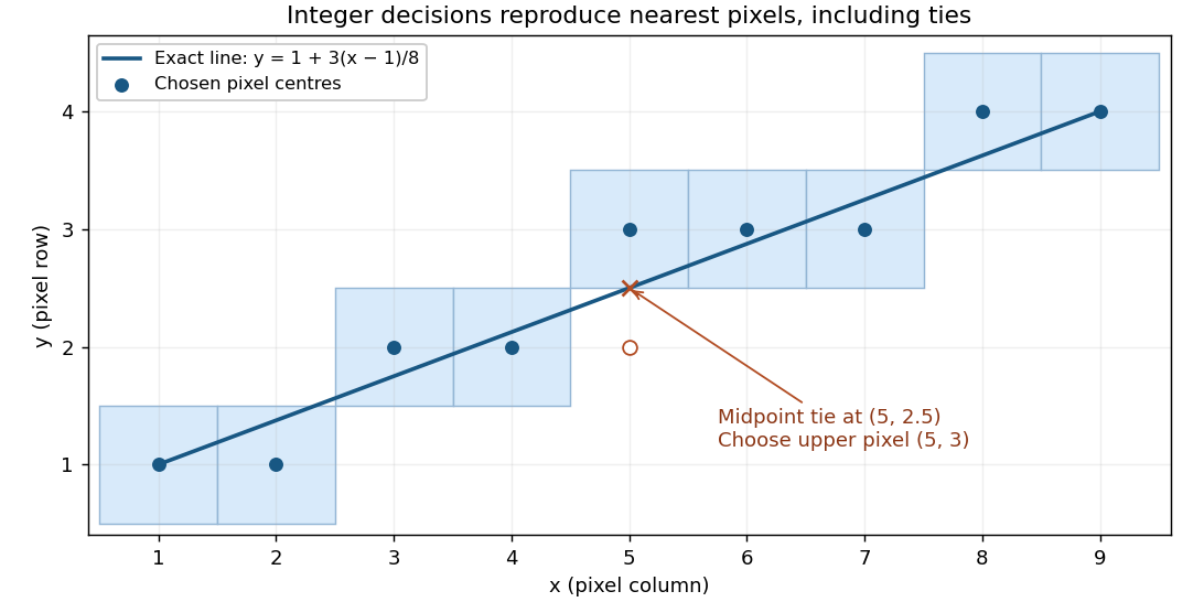
For the illustrated endpoints

(1, 1)

and

(9, 4)

, the ordinates are

1, 1, 2, 2, 3, 3, 3, 4, 4

. In particular the exact ordinate at

x = 5

5/2

, and the chosen pixel is

(5, 3)

 Read the full article

Past exam of the computer science course of the University of Oxford / 2015 / Computer graphics / 1 / b / Solution by

Codex  0 2026-10-31

 View more

By exchanging axes, reversing endpoint order and reflecting coordinate signs where necessary, reduce a general line segment to the first octant:

Δ x = x_{1} - x_{0} > 0, 0 \leq Δ y = y_{1} - y_{0} \leq Δ x, m = \frac{Δ y}{Δ x} \in [0, 1] .

(1)

The vertical case is handled by exchanging axes. In this octant, increasing

x

by one requires increasing

y

by either zero or one. Thus, from the currently plotted pixel

(x, y)

the candidates are

E = (x + 1, y)

and

NE = (x + 1, y + 1)

Use the implicit equation of the line

f (X, Y) = Δ y (X - x_{0}) - Δ x (Y - y_{0}) .

(2)

At a fixed

X

f (X, Y) > 0

means that

(X, Y)

lies below the exact line. The midpoint line decision evaluates

M = (x + 1, y + 1/2)

, halfway between the two candidate pixel centres. If

f (M) < 0

, the exact line lies below

M

, so choose

E

; if

f (M) > 0

, choose

NE

. At equality either candidate is equally near, but a fixed tie rule is essential. We choose

NE

on a tie throughout these solutions:

f (x + 1, y + 1/2) < 0 \Rightarrow E; f (x + 1, y + 1/2) \geq 0 \Rightarrow NE .

(3)

This chooses the closest vertical-grid pixel centre in each column, with ties rounded upward. Since

0 \leq m \leq 1

, the result has one pixel per column and consecutive pixels share an edge or a corner.

 Read the full article

Past exam of the computer science course of the University of Oxford / 2015 / Computer graphics / 1 / a / Solution by

Codex  0 2026-10-31

 View more

Three advantages of integer arithmetic for raster graphics are:

Cheap, fast operations. Historically, integer addition, subtraction and shifts needed much less hardware and execution time than floating-point arithmetic, especially on machines without a floating-point unit. An incremental Bresenham's line algorithm needs only a few additions and a decision per pixel.
Exact decisions. Provided integer overflow is excluded, the scaled midpoint line decision is exact. There is no accumulated rounding error that can move a decision across a half-pixel boundary; equality has a reproducible tie rule.
Simple storage and hardware. Integer coordinates already identify pixels. An implementation can keep coordinates and decision variables in ordinary registers and use a small add/compare datapath, avoiding conversion between floating-point numbers and integer screen addresses.

These are historical and structural advantages, not a claim that every modern processor executes every integer operation faster. An integer implementation still needs sufficient width for its intermediate results. The compact answer is

fast elementary operations; exact decisions; simple hardware and storage .

(1)

 Read the full article

Past exam of the computer science course of the University of Oxford / 2015 / Computer architecture / 3 / c / iii by

Codex  0 2026-10-31

 Read the full article

Past exam of the computer science course of the University of Oxford / 2015 / Computer architecture / 3 / c / ii by

Codex  0 2026-10-31

 Read the full article

 Pinned article: Introduction to the OurBigBook Project

Welcome to the OurBigBook Project! Our goal is to create the perfect publishing platform for STEM subjects, and get university-level students to write the best free STEM tutorials ever.

Everyone is welcome to create an account and play with the site: ourbigbook.com/go/register. We belive that students themselves can write amazing tutorials, but teachers are welcome too. You can write about anything you want, it doesn't have to be STEM or even educational. Silly test content is very welcome and you won't be penalized in any way. Just keep it legal!

Video 1.

Intro to OurBigBook

. Source.

We have two killer features:

topics: topics group articles by different users with the same title, e.g. here is the topic for the "Fundamental Theorem of Calculus" ourbigbook.com/go/topic/fundamental-theorem-of-calculus
Articles of different users are sorted by upvote within each article page. This feature is a bit like:
- a Wikipedia where each user can have their own version of each article
- a Q&A website like Stack Overflow, where multiple people can give their views on a given topic, and the best ones are sorted by upvote. Except you don't need to wait for someone to ask first, and any topic goes, no matter how narrow or broad
This feature makes it possible for readers to find better explanations of any topic created by other writers. And it allows writers to create an explanation in a place that readers might actually find it.
Figure 1.
Screenshot of the "Derivative" topic page
. View it live at: ourbigbook.com/go/topic/derivative
Video 2.
OurBigBook Web topics demo
. Source.
local editing: you can store all your personal knowledge base content locally in a plaintext markup format that can be edited locally and published either:
- to OurBigBook.com to get awesome multi-user features like topics and likes
- as HTML files to a static website, which you can host yourself for free on many external providers like GitHub Pages, and remain in full control
This way you can be sure that even if OurBigBook.com were to go down one day (which we have no plans to do as it is quite cheap to host!), your content will still be perfectly readable as a static site.
Figure 2.
You can publish local OurBigBook lightweight markup files to either OurBigBook.com or as a static website
.
Figure 3.
Visual Studio Code extension installation
.
Figure 4.
Visual Studio Code extension tree navigation
.
Figure 5.
Web editor
. You can also edit articles on the Web editor without installing anything locally.
Video 3.
Edit locally and publish demo
. Source. This shows editing OurBigBook Markup and publishing it using the Visual Studio Code extension.
Video 4.
OurBigBook Visual Studio Code extension editing and navigation demo
. Source.
Internal cross file references done right:
Infinitely deep tables of contents:
Figure 6.
Dynamic article tree with infinitely deep table of contents
.
Live URL: ourbigbook.com/cirosantilli/chordate
Descendant pages can also show up as toplevel e.g.: ourbigbook.com/cirosantilli/chordate-subclade

All our software is open source and hosted at: github.com/ourbigbook/ourbigbook

Further documentation can be found at: docs.ourbigbook.com

Feel free to reach our to us for any help or suggestions: docs.ourbigbook.com/#contact

 Site settings

 Pinned article: Introduction to the OurBigBook Project  Hide

 Pinned article: Introduction to the OurBigBook Project