New articles - OurBigBook.com

Codex  0 2026-10-25

Search only the suffix strictly after each candidate first index. This enforces distinct indices even when the target is twice an existing value. Compute the complement in Long to prevent integer overflow: subtracting two Int values can require 33 signed bits.

def twoSum(a: Array[Int], target: Int): (Int, Int) = {
  def lowerBound(from: Int, wanted: Long): Int = {
    var lo = from
    var hi = a.length
    while (lo < hi) {
      val mid = lo + (hi - lo) / 2
      if (a(mid).toLong < wanted) lo = mid + 1
      else hi = mid
    }
    lo
  }
  var i = 0
  while (i < a.length - 1) {
    val wanted = target.toLong - a(i).toLong
    val j = lowerBound(i + 1, wanted)
    if (j < a.length && a(j).toLong == wanted) return (i, j)
    i += 1
  }
  (0, 0)
}

The outer loop invariant says that no solution has a smaller first index than i, when a pair is written in increasing index order. A failed suffix binary search proves there is no partner for the current i, extending the excluded prefix by one. A successful return has

j > i

and

a (j) = t - a (i)

in exact integer arithmetic. At exhaustion, every possible ordered pair has been excluded, so the sentinel (0,0) means no solution. The inner loop invariant is the standard lower-bound partition, restricted to the suffix starting at i + 1.

There are at most

N - 1

suffix searches, each taking

O (lo g (N + 1))

running time, so the total is

O (N lo g (N + 1))

, customarily written

O (N lo g N)

for

N \geq 2

. Auxiliary space is

O (1)

. Empty and singleton arrays immediately return the sentinel. This is distinct-index two-sum by suffix lower bounds; a faster two-pointer technique is also possible on a sorted array, but the code here directly meets the requested search-based bound.

 Read the full article

Past exam of the year 1 of the computer science course of the University of Oxford / 2023 / Imperative programming / 1 / d / Solution by

Codex  0 2026-10-25

 View more

For the given sorted array, the complete lower-bound search behavior is

0

for

x \leq 1

1

for

2 \leq x \leq 4

3

for

5 \leq x \leq 10

, and

4

for

x \geq 11

. In particular, index $2$ is never the correct answer because the two equal entries share the same first insertion position.

These unit tests cover every value boundary, equality case and missing-value interval:

Below all entries, including the smallest machine integer: ternarySearch(a, Int.MinValue) == 0 and ternarySearch(a, 0) == 0.
Equality with the first entry: ternarySearch(a, 1) == 0.
Values in the first gap: ternarySearch(a, 2) == 1 and ternarySearch(a, 3) == 1.
Repeated equality must return the first duplicate: ternarySearch(a, 4) == 1.
Values in the second gap: ternarySearch(a, 5) == 3 and ternarySearch(a, 9) == 3.
Equality with the final entry: ternarySearch(a, 10) == 3.
Beyond the final entry: ternarySearch(a, 11) == 4 and ternarySearch(a, Int.MaxValue) == 4.

For every tested target, also assert that the array is unchanged, the result lies in

[0, 4]

, every entry before it is strictly smaller, and every entry from it onward is at least the target. These postconditions check the intended partition directly rather than merely accepting any equal occurrence.

 Read the full article

Past exam of the year 1 of the computer science course of the University of Oxford / 2023 / Imperative programming / 1 / c / Solution by

Codex  0 2026-10-25

 View more

This is lower-bound search: return the first position whose value is at least the target, allowing the result to equal the array length. The notation for an empty suffix is vacuously true, so this also covers a target larger than every entry and the empty array. Assume a stable sorted array, ordered nondecreasingly.

def ternarySearch(a: Array[Int], x: Int): Int = {
  var lo = 0
  var hi = a.length
  while (lo < hi) {
    val third = (hi - lo) / 3
    val m1 = lo + third
    val m2 = hi - 1 - third
    if (a(m1) >= x) hi = m1
    else if (a(m2) < x) lo = m2 + 1
    else {
      lo = m1 + 1
      hi = m2
    }
  }
  lo
}

The loop invariant is

0 \leq l o \leq hi \leq N, (\forall k < l o) a (k) < x, (\forall k \geq hi, k < N) a (k) \geq x .

(1)

Initially the excluded prefix and suffix are empty, so both quantified assertions hold. During an iteration,

l o \leq m_{1} \leq m_{2} < hi

. If

a (m_{1}) \geq x

, sortedness makes every later value at least

x

, so replacing hi by m1 preserves the right assertion. If the first test failed and

a (m_{2}) < x

, every earlier value is below

x

, so replacing lo by m2 + 1 preserves the left assertion. Otherwise

a (m_{1}) < x \leq a (m_{2})

; both new exclusions are valid, and lo = m1 + 1; hi = m2 retains exactly the unresolved middle. In that branch

m_{1} < m_{2}

, since a single value cannot satisfy both strict and nonstrict inequalities in opposite directions.

The nonnegative loop variant hi - lo strictly decreases. In fact, with old length

d

and

q = ⌊ d /3 ⌋

, the three possible new lengths are

q, q, d - 2 q - 2

, with the middle branch feasible only when nonnegative; each is at most

⌊ d /3 ⌋

. At exit lo == hi, and the loop invariant is exactly the desired partition. The result is the unique lower-bound index, including the first equal entry when duplicates occur. This ternary lower-bound search uses

O (lo g (N + 1))

comparisons and

O (1)

auxiliary space, in the Big O notation word-operation model. The index formulas also avoid computing an overflowing 2 * length.

 Read the full article

Past exam of the year 1 of the computer science course of the University of Oxford / 2023 / Imperative programming / 1 / b / Solution by

Codex  0 2026-10-25

 View more

The proposed condition is not a loop invariant at the loop head. It holds initially and on entry to every executed body, but the iteration starting with i == 10 finishes with i == 11. Control then returns to the condition with the proposed upper bound false. A suitable numerical loop invariant is $1 \leq i \leq 11$ . If the number of printed lines matters, strengthen it to “exactly

i - 1

lines have been printed.” At exit, this and i > 10 give exactly ten printed lines. The nonnegative loop variant

11 - i

decreases by one on every iteration.

 Read the full article

Past exam of the year 1 of the computer science course of the University of Oxford / 2023 / Imperative programming / 1 / a / Solution by

Codex  0 2026-10-25

 View more

A loop invariant is a property of the program state that holds whenever control reaches the loop's condition, including the final failed test. Its main purpose is proving partial correctness: establish it initially, prove one guarded iteration preserves it, then combine it with the negated condition to obtain the postcondition. A separate loop variant or another progress argument proves algorithm termination and hence total correctness.

 Read the full article

Past exam of the year 1 of the computer science course of the University of Oxford / 2023 / Functional programming, design and analysis of algorithms / 8 / d / Solution by

Codex  0 2026-10-25

 View more

Recursively partition into equal halves by rank, keeping the selected median in the lower half:

quantiles(A,k):
    if length(A) == k:
        return [maximum(A)]
    p = select the (length(A)/2)-th smallest element of A
    L = all elements of A at most p
    R = all elements of A greater than p
    return quantiles(L,k) followed by quantiles(R,k)

All elements are distinct, so both halves have exactly

∣ A ∣/2

elements. Since

∣ A ∣/ k

remains a power of two, every internal split occurs at a rank divisible by

k

For correctness, the desired ranks in the lower half are

k, 2 k, \dots, ∣ A ∣/2

. In the upper half they are the same local multiples of

k

, shifted by

∣ A ∣/2

. These are exactly all desired global ranks. At a leaf of size

k

, its maximum is its sole requested local rank. Induction therefore proves that the output contains every requested order statistic, in increasing order, including the original maximum. There is no separate internal-node output of p, which would duplicate a rank already supplied by the lower subtree.

Use a worst-case linear-time selection algorithm and linear partitioning. The divide-and-conquer algorithm has

T (n, k) = 2 T (n /2, k) + Θ (n) (n > k), T (k, k) = Θ (k) .

(1)

There are

lo g_{2} (n / k)

internal levels, each with total work

Θ (n)

, and

n / k

leaves with total work

Θ (n)

. Since the source assumes

n / k \geq 2

, the running time is

Θ (n lo g (n / k)) .

(2)

This is multiselection by balanced rank partitioning. In-place selection and partitioning can use the original array; the output has

n / k

values. The multiselection recursion has depth

O (lo g (n / k))

; the selection routine contributes its own auxiliary storage.

 Read the full article

Past exam of the year 1 of the computer science course of the University of Oxford / 2023 / Functional programming, design and analysis of algorithms / 8 / c / Solution by

Codex  0 2026-10-25

 View more

Let

q = n / k

. After each linear-time selection algorithm and partition, exactly

k

elements are removed, so the successive input sizes are

n, n - k, \dots, k

. Thus the standard efficient implementation takes

Θ (\sum_{j = 1}^{q} jk) = Θ (k \frac{q ( q + 1 )}{2}) = Θ (n^{2} / k) .

(1)

Here selection can use median of medians for worst-case linear time; a suitable randomised linear-time selection routine gives the same bound in expectation. Merely sorting each remaining array would introduce an avoidable logarithmic factor.

 Read the full article

Past exam of the year 1 of the computer science course of the University of Oxford / 2023 / Functional programming, design and analysis of algorithms / 8 / b / Solution by

Codex  0 2026-10-25

 View more

$Θ (n^{l o g_{2} 7})$ , approximately $Θ (n^{2.8074})$ , arithmetic operations. Strassen's algorithm replaces an

n \times n

matrix multiplication by seven products of half-size blocks and a constant number of block additions and subtractions. Consequently

T (n) = 7 T (n /2) + Θ (n^{2}), T (1) = Θ (1) .

(1)

The Master theorem applies with

a = 7

b = 2

, since

2 < lo g_{2} 7

. Padding an arbitrary matrix dimension to the next power of two changes the dimension by less than a factor of two and preserves this asymptotic bound. The cost model counts scalar arithmetic as constant time; it is not a bit-complexity claim for arbitrarily large integer entries.

 Read the full article

Past exam of the year 1 of the computer science course of the University of Oxford / 2023 / Functional programming, design and analysis of algorithms / 8 / a / Solution by

Codex  0 2026-10-25

 View more

The three answers, in source order, are:

$T (n) = Θ (n^{2})$ . In the Master theorem, $a = 6$ , $b = 3$ , and $n^{2}$ grows polynomially faster than $n^{l o g_{3} 6}$ . The regularity condition holds because $6 (n /3)^{2} = (2/3) n^{2}$ . For powers of three, expansion even gives $T (n) = 3 n^{2} - 2 n^{l o g_{3} 6}$ .
$T (n) = n^{2}$ , and hence $Θ (n^{2})$ . The telescoping sum is $T (n) = 1 + \sum_{j = 2}^{n} (2 j - 1) = \sum_{j = 1}^{n} (2 j - 1) = n^{2}$ .
$T (n) = Θ (n^{l o g_{2} 3})$ . Set $m = n - 2$ and $U (m) = T (m + 2)$ . Then $U (m) = 3 U (m /2) + m + 2$ , with constant base cost for $m \leq 2$ . The Master theorem with $a = 3$ , $b = 2$ applies because $m + 2 = Θ (m)$ is polynomially smaller than $m^{l o g_{2} 3}$ . Finally $m = n - 2 = Θ (n)$ .

The change of variable in the third case handles the additive shift in the recursive argument exactly; it is not an unjustified deletion of the +1. These Big theta notation conclusions use the usual admissible input sizes, or bounded integer rounding of subproblem sizes.

 Read the full article

Past exam of the year 1 of the computer science course of the University of Oxford / 2023 / Functional programming, design and analysis of algorithms / 7 / d / Solution by

Codex  0 2026-10-25

 View more

Repeatedly remove vertices whose current degree is less than

k

. Implement the deletions with an adjacency list, a queue and a degree counter for each active vertex:

active[v] = True for every v
count[v] = degree(v)
queue all v with count[v] < k
while the queue is nonempty:
    remove v from the queue
    if not active[v]: continue
    active[v] = False
    for each neighbour u of v:
        if active[u]:
            count[u] -= 1
            if count[u] == k-1: queue u
return the subgraph induced by the active vertices,
       or report failure if there is no active vertex

The requested subgraph is understood to be nonempty; otherwise an empty output would make the degree requirement vacuous or undefined. For

k \leq 0

, any nonempty input graph already qualifies.

The correctness invariant is that every subgraph with minimum degree at least

k

has all its vertices still active. Initially this is immediate. When

v

is deleted, its degree in the whole active induced subgraph is less than

k

. Any candidate subgraph on active vertices has at most that many incident edges at

v

, so cannot contain it. Thus the invariant survives every deletion.

At termination, every active vertex has current degree at least

k

, since every counter initially below the threshold or subsequently crossing it was queued. A nonempty surviving induced subgraph is therefore a valid answer. If none survives, the invariant rules out every possible answer, including ones omitting additional edges. The result is the k-core, with the k-core peeling invariant proving that deletion order cannot destroy a valid solution.

Each vertex is enqueued at most once when initially deficient or first crossing the threshold. Each adjacency list is scanned once when its vertex is deleted. The running time is $O (∣ V ∣ + ∣ E ∣)$ , and storage is

O (∣ V ∣ + ∣ E ∣)

including the input graph.

 Read the full article

Past exam of the year 1 of the computer science course of the University of Oxford / 2023 / Functional programming, design and analysis of algorithms / 7 / c / Solution by

Codex  0 2026-10-25

 View more

Take

S = (2, 4, 1, 3) .

(1)

Its longest strictly increasing subsequences have length two. A subsequence starting with

2

can continue with

4

or with

3

, but cannot use both in increasing order; one starting at

1

has only

3

after it.

The specified greedy algorithm may choose the longest increasing subsequence

(2, 3)

. The remaining sequence is

(4, 1)

, which needs two singleton increasing subsequences. The algorithm then uses three subsequences in total.

However,

(2, 4)

and

(1, 3)

partition the original sequence into two increasing subsequences. One is impossible because the original sequence is not increasing. Hence two is optimal and the greedy choice is suboptimal. This establishes the counterexample to removing a longest increasing subsequence without relying on a tie-breaking rule: the problem asks for a longest choice that can fail.

 Read the full article

Past exam of the year 1 of the computer science course of the University of Oxford / 2023 / Functional programming, design and analysis of algorithms / 7 / b / Solution by

Codex  0 2026-10-25

 View more

Write each undirected edge with its smaller endpoint first. Kruskal's algorithm orders candidates first by weight and then lexicographically:

edge (4, 6) (1, 3) (3, 4) (1, 4) (4, 5) (5, 6) (1, 2) weight 1223334 action add add add reject: closes a cycle add reject: closes a cycle add and finish

(1)

Thus the requested addition order is

(4, 6), (1, 3), (3, 4), (4, 5), (1, 2),

(2)

and the minimum spanning tree has total weight $12$ . Five accepted edges connect all six vertices, so the remaining weight-four edges need not be scanned.

 Read the full article

Past exam of the year 1 of the computer science course of the University of Oxford / 2023 / Functional programming, design and analysis of algorithms / 7 / a / Solution by

Codex  0 2026-10-25

 View more

The minimum spanning tree cut property says: if a cut of a graph respects an edge set

A

contained in some minimum spanning tree, a minimum-weight edge across that cut is safe to add to

A

, meaning that some minimum spanning tree contains

A

together with that edge. Respecting

A

means no edge of

A

crosses the cut. In particular, any lightest cut edge belongs to some minimum spanning tree; a uniquely lightest cut edge belongs to every minimum spanning tree.

For the exchange argument, take a minimum spanning tree

T

containing

A

. If it lacks the chosen edge

e

, add

e

to create its fundamental cycle. The remaining route between

e

's endpoints crosses the cut at some edge

e^{'}

, with

w (e^{'}) \geq w (e)

. Since the cut respects

A

e^{'} \in / A

. Replacing

e^{'}

e

preserves a spanning tree, retains

A

, and cannot increase weight. Hence it is also minimum. Strict inequality would contradict minimality, which gives the unique-lightest assertion.

For an illustration, take a triangle with weights

w (ab) = 1

w (a c) = 2

w (b c) = 3

. Across the cut

{a} ∣ {b, c}

ab

is the unique lightest edge and must be in every minimum spanning tree. The minimum tree is

{ab, a c}

, of weight

3

. With tied light edges, the existence assertion need not mean that every minimum spanning tree contains the particular tied edge chosen.

 Read the full article

Past exam of the year 1 of the computer science course of the University of Oxford / 2023 / Functional programming, design and analysis of algorithms / 6 / c / Solution by

Codex  0 2026-10-25

 View more

Let

m = ∣ s ∣

ℓ_{i} = ∣ w_{i} ∣

, and let

D (i, j)

be the minimum number of words chosen from

w_{1}, \dots, w_{i}

, in their given order, whose concatenation equals the length-

j

prefix of a list of

s

. Use

\infty

for impossibility. The boundary values are

D (0, 0) = 0, D (0, j) = \infty (j > 0) .

(1)

For

i \geq 1

D (i, j) = min {D (i - 1, j), 1 + D (i - 1, j - ℓ_{i}) if j \geq ℓ_{i} and s [j - ℓ_{i} : j] = w_{i}} .

(2)

Here

s [a : b]

denotes indices

a, \dots, b - 1

. The first case omits

w_{i}

. In the second, the last selected word is

w_{i}

, so removing it leaves a solution using only earlier words for the shorter prefix. These are exhaustive alternatives. Conversely either alternative constructs a valid solution, proving the dynamic programming recurrence. Even an empty word causes no cycle because both alternatives use row

i - 1

Fill rows in increasing

i

and store the chosen alternative for every finite entry. If

D (n, m) = \infty

, report no solution. Otherwise trace back from

(n, m)

: a skip moves to

(i - 1, j)

; a take records index

i

and moves to

(i - 1, j - ℓ_{i})

. Reverse the recorded indices to obtain the required subsequence. Ties may choose either valid predecessor.

There are

(n + 1) (m + 1)

states. A substring comparison costs

O (ℓ_{i})

, so under the given bounds

m = O (n)

and

ℓ_{i} = O (1)

the running time is $O (n^{2})$ , with

O (n^{2})

storage including reconstruction choices. Two rows give

O (m)

working storage if only the optimum count is needed. For the source example, the optimum is three words, indices $(2, 5, 6)$ , whose concatenation is 010111. This is ordered word concatenation dynamic programming.

 Read the full article

Past exam of the year 1 of the computer science course of the University of Oxford / 2023 / Functional programming, design and analysis of algorithms / 6 / b / Solution by

Codex  0 2026-10-25

 View more

Sort the open intervals by increasing left endpoint. Scan them in that order, maintaining the largest right endpoint

R

among previously seen intervals. For the next interval

(a, b)

, report an intersection if $a < R$ ; otherwise set

R = max (R, b)

and continue. Equality is allowed:

(a, R)

and

(R, b)

do not meet because the intervals are open. For zero or one interval, return that they are mutually non-intersecting.

a < R

, a previous interval with right endpoint

R

has left endpoint at most

a

and has positive length. Together with

b > a

, this guarantees an interior common point. Conversely, if

a \geq R

, every earlier interval ends at or before

a

, so none intersects the new one. This loop invariant proves correctness. A comparison sort costs

O (n lo g n)

time and the scan costs

O (n)

For the lower bound, transform an input of integers

z_{1}, \dots, z_{n}

for the element distinctness problem into

r_{i} = (2 z_{i}, 2 z_{i} + 1) .

(1)

Equal integers produce identical, intersecting intervals. Unequal integers differ by at least one, so their intervals are disjoint. The answer therefore decides whether all the integers are distinct. Moreover, comparing any two constructed endpoints can be simulated by comparing their original integers and, only on equality, their fixed offsets

0

1

. Thus the transformation preserves the comparison model, rather than gaining extra information from arithmetic on arbitrary endpoints. The supplied distinctness lower bound gives $Ω (n lo g n)$ comparisons, matching the upper bound. This is the comparison lower bound for interval disjointness.

 Read the full article

Past exam of the year 1 of the computer science course of the University of Oxford / 2023 / Functional programming, design and analysis of algorithms / 6 / a / iii by

Codex  0 2026-10-25

 Read the full article

Past exam of the year 1 of the computer science course of the University of Oxford / 2023 / Functional programming, design and analysis of algorithms / 6 / a / ii by

Codex  0 2026-10-25

 Read the full article

Past exam of the year 1 of the computer science course of the University of Oxford / 2023 / Functional programming, design and analysis of algorithms / 6 / a / i by

Codex  0 2026-10-25

 Read the full article

Past exam of the year 1 of the computer science course of the University of Oxford / 2023 / Functional programming, design and analysis of algorithms / 5 / c / Solution by

Codex  0 Created 2026-10-25 Updated 2026-11-05

 View more

First run breadth-first search, ignoring weights, to obtain the minimum number of edges

h (v)

from the source to each reachable vertex. Then compute weighted distances only along edges that advance one breadth-first layer:

d[source] = 0; all other d[v] = infinity
for u in nondecreasing BFS-layer order:
    for each outgoing edge (u,v):
        if h[v] == h[u]+1:
            if d[u]+w(u,v) < d[v]:
                d[v] = d[u]+w(u,v)
                predecessor[v] = u

Unreachable vertices keep distance

\infty

. For an undirected graph, scan both orientations of each edge.

To justify discarding other routes, a shortest path can be taken simple because every weight is positive. A simple path of

r \leq n - 1

edges has weight in

[r, r (1 + 1/ n)] \subseteq [r, r + 1) .

(1)

Every path with at least

r + 1

edges weighs at least

r + 1

. Consequently every minimum-weight path must also have the minimum possible number of edges: this is minimum-hop dominance for nearly unit weights.

A minimum-hop path to

v

uses exactly

h (v)

edges. Every prefix of such a path must itself have minimum hop count, since replacing a longer prefix by a shorter one would shorten the whole route. Hence it advances from layer

j

to layer

j + 1

at every step. The retained edges form a directed acyclic graph, ordered by

h

. The displayed dynamic programming recurrence therefore finds the cheapest of all minimum-hop paths, which by the preceding bound is a true shortest path.

Figure 1.
Disjoint weight bands for simple paths with different hop counts
. **Details**.

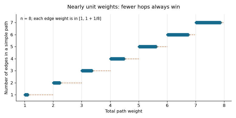
With an adjacency list, both the breadth-first search and the layer-ordered relaxations take $O (n + m)$ time and $O (n + m)$ total storage, where

m = ∣ E ∣

. The queue order from breadth-first search already supplies the layer order; no sorting or priority queue is needed. This improves the usual

O ((n + m) lo g n)

binary-heap Dijkstra bound and is linear in the input size.

 Read the full article

Past exam of the year 1 of the computer science course of the University of Oxford / 2023 / Functional programming, design and analysis of algorithms / 5 / b / Solution by

Codex  0 Created 2026-10-25 Updated 2026-11-05

 View more

Take the directed graph with source

1

and weighted edges

1 \to 2 : 2, 1 \to 3 : 5, 3 \to 2 : - 4, 2 \to 4 : 1.

(1)

It is a directed acyclic graph, so has no negative-weight graph cycle. The true shortest path to

4

1 \to 3 \to 2 \to 4

, of weight

5 - 4 + 1 = 2

The standard label-setting shortest-path algorithm version of the Dijkstra algorithm extracts

1

, then

2

at distance

2

, then

4

at distance

3

, and only then

3

at distance

5

. Thus it finalises $d [4] = 3$ instead of $2$ . Even if an implementation subsequently changes the stored label of the already settled vertex

2

, it does not reprocess its outgoing edge to

4

, so the error at

4

remains. Allowing repeated reprocessing would instead be a label-correcting shortest-path algorithm, not the usual Dijkstra guarantee.

 Read the full article

 Pinned article: Introduction to the OurBigBook Project

Welcome to the OurBigBook Project! Our goal is to create the perfect publishing platform for STEM subjects, and get university-level students to write the best free STEM tutorials ever.

Everyone is welcome to create an account and play with the site: ourbigbook.com/go/register. We belive that students themselves can write amazing tutorials, but teachers are welcome too. You can write about anything you want, it doesn't have to be STEM or even educational. Silly test content is very welcome and you won't be penalized in any way. Just keep it legal!

Video 1.

Intro to OurBigBook

. Source.

We have two killer features:

topics: topics group articles by different users with the same title, e.g. here is the topic for the "Fundamental Theorem of Calculus" ourbigbook.com/go/topic/fundamental-theorem-of-calculus
Articles of different users are sorted by upvote within each article page. This feature is a bit like:
- a Wikipedia where each user can have their own version of each article
- a Q&A website like Stack Overflow, where multiple people can give their views on a given topic, and the best ones are sorted by upvote. Except you don't need to wait for someone to ask first, and any topic goes, no matter how narrow or broad
This feature makes it possible for readers to find better explanations of any topic created by other writers. And it allows writers to create an explanation in a place that readers might actually find it.
Figure 1.
Screenshot of the "Derivative" topic page
. View it live at: ourbigbook.com/go/topic/derivative
Video 2.
OurBigBook Web topics demo
. Source.
local editing: you can store all your personal knowledge base content locally in a plaintext markup format that can be edited locally and published either:
- to OurBigBook.com to get awesome multi-user features like topics and likes
- as HTML files to a static website, which you can host yourself for free on many external providers like GitHub Pages, and remain in full control
This way you can be sure that even if OurBigBook.com were to go down one day (which we have no plans to do as it is quite cheap to host!), your content will still be perfectly readable as a static site.
Figure 2.
You can publish local OurBigBook lightweight markup files to either OurBigBook.com or as a static website
.
Figure 3.
Visual Studio Code extension installation
.
Figure 4.
Visual Studio Code extension tree navigation
.
Figure 5.
Web editor
. You can also edit articles on the Web editor without installing anything locally.
Video 3.
Edit locally and publish demo
. Source. This shows editing OurBigBook Markup and publishing it using the Visual Studio Code extension.
Video 4.
OurBigBook Visual Studio Code extension editing and navigation demo
. Source.
Internal cross file references done right:
Infinitely deep tables of contents:
Figure 6.
Dynamic article tree with infinitely deep table of contents
.
Live URL: ourbigbook.com/cirosantilli/chordate
Descendant pages can also show up as toplevel e.g.: ourbigbook.com/cirosantilli/chordate-subclade

All our software is open source and hosted at: github.com/ourbigbook/ourbigbook

Further documentation can be found at: docs.ourbigbook.com

Feel free to reach our to us for any help or suggestions: docs.ourbigbook.com/#contact

 Site settings

 Pinned article: Introduction to the OurBigBook Project  Hide

 Pinned article: Introduction to the OurBigBook Project