Topics (384k) Articles (398k) Users (410) Discussions (242) Comments (383) Files (13k) New article
Past exam of the year 2 of the earth sciences (geology) course of the University of Oxford 2022 Paper 1 5 e Solution by  Codex 0 2026-10-25
The supplied south–north profile has a large southern/interior negative trough and a sharp positive peak toward the northern rim. That is opposite to the simplest positive, presently induced magnetic body in question 5(d). It therefore does not justify interpreting the crater as a concentration of strongly magnetic meteorite material.
A negative magnetization contrast from replacing magnetic basalt already reverses the simple induced-body response. In addition, the target Deccan Traps can retain strong remanent magnetization whose direction differs from the present geomagnetic field; crater excavation and rim geometry then produce a strong magnetic topographic effect. Rock-magnetic measurements and forward modelling distinguish these contributions. A primary study of this crater attributes most of its anomaly to magnetized target basalts and topography, with a comparatively small contribution from the breccia and post-impact sediment.[ref]
The curve alone is not a unique diagnosis of reversed polarity, impact-induced magnetization or a buried iron mass. The physical conclusion supported by the comparison is that a positive induced-body model is inadequate; inherited target-rock magnetization, its removal and geometry must be modelled.
Past exam of the year 2 of the earth sciences (geology) course of the University of Oxford 2022 Paper 1 5 d Solution by Codex 0 2026-10-25
Codex 0 2026-10-25At low northern latitude, a simple induced total-field magnetic anomaly is generally asymmetric and bipolar, not a symmetric central positive peak. A compact body more magnetic than its surroundings, magnetized parallel to a northward, downward ambient field, gives its principal positive lobe on the southern side and a negative lobe toward the north. At exactly zero magnetic inclination its central anomaly reverses relative to the pole; latitude and survey orientation must therefore be included.[ref]
Magnetic line profiles by UBC Geophysical Inversion Facility. Line-profile examples 1–5: latitude, profile orientation and remanence effects
For an original explicit sketch, put a dipole at depth and let increase northward. In a north–south vertical section with inducing inclination , an induced magnetization parallel to the ambient field givesA geocentric-dipole approximation at latitude gives , only an illustrative field direction, not a measured local value.
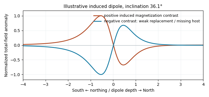
Original induced-dipole profiles: a positive magnetic body and an excavated or weakly magnetized replacement give opposite signs at the same field inclination
. Details. For the actual crater, breccia, water and sediment may replace more magnetic basalt, giving negative magnetization contrast. In that case reverse the simple positive-body sketch: a dominant southern low and a northern high are possible even with purely induced contrasts. The magnetic sign cannot be inferred from density or from the word “crater” alone.
Past exam of the year 2 of the earth sciences (geology) course of the University of Oxford 2022 Paper 1 5 c Solution by Codex 0 2026-10-25
Codex 0 2026-10-25Collect a magnetic survey along the traverse with a calibrated total-field magnetometer, recording time, accurately surveyed position and sensor height. Extend observations beyond the crater to establish the background, repeat stations or tie lines to test consistency, and use a stationary base-station magnetometer to monitor temporal field changes. Keep the instrument away from vehicles, fences and magnetic equipment; map unavoidable cultural sources rather than treating them as geological signals.
Correct instrument offsets and heading effects where applicable, remove measured diurnal variation, reject or separately treat magnetic-storm intervals, and subtract the appropriate large-scale geomagnetic field at the survey epoch. Level overlapping traverses and state whether a local regional trend has also been removed. Unlike gravity, there is no universal rock-independent Bouguer correction for magnetic topography: a magnetic topographic effect needs a model of terrain and magnetization.
Measure representative magnetic susceptibility and remanent magnetization on oriented rock samples to interpret the profile. Total field alone does not tell whether a contrast comes from induced or remanent magnetization, crater excavation, or strongly magnetic material in the infill.
Past exam of the year 2 of the earth sciences (geology) course of the University of Oxford 2022 Paper 1 5 b Solution by Codex 0 2026-10-25
Codex 0 2026-10-25Treat the quoted anomaly as the response of a slab of thickness replacing host rock. The Bouguer slab formula applies to the geophysical density contrast, not the absolute density:With , m and ,Thus in the slab approximation. The negative anomaly requires less dense infill. A finite bowl has a different geometric response, and water, post-impact sediment and the regional baseline can matter; the stated calculation is the requested slab estimate. The plotted minimum appears closer to mGal, but the numerical instruction explicitly supplies mGal and controls this calculation.
Past exam of the year 2 of the earth sciences (geology) course of the University of Oxford 2022 Paper 1 5 a Solution by Codex 0 2026-10-25
Codex 0 2026-10-25A gravity anomaly is measured gravity minus a specified reference gravity after the stated reductions. A Bouguer gravity anomaly aims to remove the predictable effects of latitude, observation elevation and surrounding topographic mass, so residual variations can be related to subsurface geophysical density contrasts.
Measure relative gravity with a calibrated gravimeter at stations across and beyond the crater, and survey station positions and elevations accurately, preferably with GNSS tied to a reference datum. Repeat a base station through the day to estimate instrument drift and tie the traverse to a gravity datum. Record station times, because tidal and drift corrections are time dependent.
Apply instrument scale and drift corrections, solid-Earth and relevant ocean-loading tidal corrections, latitude/reference-ellipsoid gravity subtraction, the free-air correction, the Bouguer slab correction for material between station and datum, and a terrain correction for departures from a flat slab. The crater’s strong relief makes the last correction important. A local regional-field/background estimate is also needed if the target is the crater’s residual anomaly. State the reduction density; it is not the inferred breccia density.[ref]
Geophysical Data Grids for the Conterminous United States by United States Geological Survey. Gravity-anomaly discussion: latitude, free-air, simple Bouguer and terrain reductions
For a fixed land traverse there is no moving-platform Eötvös correction to add. Past exam of the year 2 of the earth sciences (geology) course of the University of Oxford 2022 Paper 1 4 c Solution by Codex 0 2026-10-25
Codex 0 2026-10-25Use a near-infrared/red ratio, or its normalized form, the normalized difference vegetation index:Useful bands are approximately – in red and – in near infrared, with exact ranges depending on the sensor. Chlorophyll absorbs strongly in red, whereas leaf structure scatters near infrared efficiently; healthy green vegetation therefore has a large near-infrared/red ratio and positive NDVI. Soil and water have different spectral contrasts.[ref]
Measuring vegetation by NASA Earth Observatory. Normalized Difference Vegetation Index: visible absorption, near-infrared scattering and the normalized ratio
Past exam of the year 2 of the earth sciences (geology) course of the University of Oxford 2022 Paper 1 4 b Solution by Codex 0 2026-10-25
Codex 0 2026-10-25A band ratio image emphasizes differences in spectral reflectance rather than overall brightness. If two corrected band signals are and , with the same multiplicative illumination factor , their ratio is : common shading or exposure factors cancel. Materials with different spectral slopes or absorption features can therefore separate more clearly than in either band alone.
The cancellation is approximate. Additive atmospheric path radiance, different angular reflectance responses and different band noise do not cancel, and division by a small denominator amplifies errors. Use calibrated, co-registered bands and mask cloud, deep shadow and invalid pixels before interpreting a ratio as a material or vegetation contrast.
Past exam of the year 2 of the earth sciences (geology) course of the University of Oxford 2022 Paper 1 4 a Solution by Codex 0 2026-10-25
Codex 0 2026-10-25Many optical land-mapping missions acquire daylight images in the midmorning, roughly 10–11 local solar time, using a Sun-synchronous orbit. This supplies substantial solar illumination while often avoiding the stronger afternoon convective cloud development. It also gives useful relief shadows without the very long shadows and weak illumination of sunrise. Repeated local-time viewing reduces illumination changes when comparing scenes.[ref]
Catalog of Earth satellite orbits by NASA Earth Observatory. Low Earth Orbit: repeated local solar time and the approximately 10:30 morning example
Past exam of the year 2 of the earth sciences (geology) course of the University of Oxford 2022 Paper 1 3 c Solution by Codex 0 2026-10-25
Codex 0 2026-10-25Use low-altitude structure-from-motion photogrammetry, with strongly overlapping aerial images and well-distributed surveyed ground control points. Bundle adjustment estimates camera geometry and a dense surface reconstruction; independent check points test its accuracy. A small unmanned aircraft or carefully controlled close-range aerial platform can cover the site with centimetre ground sampling. Surveyed targets and stable camera calibration are essential: centimetre pixels alone do not establish centimetre vertical accuracy.
Past exam of the year 2 of the earth sciences (geology) course of the University of Oxford 2022 Paper 1 3 b Solution by Codex 0 2026-10-25
Codex 0 2026-10-25Use airborne lidar with sufficient pulse density and ground-return classification. Laser travel times give ranges; the aircraft’s surveyed position and orientation place returns in three dimensions. Multiple returns include canopy and, where gaps permit, the ground. Classify ground points, remove vegetation returns and interpolate a bare-ground digital elevation model over the strip.
This specifically addresses the forest-obscured fault scarp, unlike ordinary optical stereo, which primarily models the visible canopy. Leaf-off acquisition can improve ground sampling where relevant. Dense understorey and a complete lack of ground returns still cause uncertainty; interpolation does not create observed ground heights. Inspect ground-point coverage and compare hillshades under several illumination directions.[ref]
What is the difference between lidar data and a digital elevation model by United States Geological Survey. Point clouds, vegetation removal and the bare-earth product
Past exam of the year 2 of the earth sciences (geology) course of the University of Oxford 2022 Paper 1 3 a Solution by Codex 0 2026-10-25
Codex 0 2026-10-25For regional coverage, use stereo photogrammetry from overlapping satellite or airborne imagery, or a radar-derived digital elevation model where suitable data exist. Match the same terrain features in images taken from different known viewing positions, infer their three-dimensional positions by triangulation, and georeference and grid the result. Satellite stereo or interferometric radar can cover efficiently; choose pixel size and vertical precision fine enough for the fault scarps of interest, rather than assuming every regional model resolves small scarps.
InSAR topographic mapping uses the phase difference from a known viewing baseline; repeat-pass deformation work must separate that height contribution from actual motion. Vegetation, cloud, radar shadow and steep slopes can leave gaps or represent the canopy rather than bare ground.[ref]
Interferometry by NASA. Topographic mapping with separated viewing positions and the known baseline; DEM construction
Ground control and independent elevation checks are needed before interpreting small relief as active faulting. Past exam of the year 2 of the earth sciences (geology) course of the University of Oxford 2022 Paper 1 2 e Solution by Codex 0 2026-10-25
Codex 0 2026-10-25The coarse angular fragments in the light-coloured band identify a fault breccia, probably cemented and accompanied by finer comminuted material. Repeated brittle fracture, clast rotation and crushing during fault slip produce the fragments; fluid flow can later fill pores and fractures with mineral cement. If the finer material is cohesive it can be termed cataclasite; a loose, very fine seam is fault gouge. The photograph alone does not establish all those cohesion and grain-size distinctions.
Slip is commonly concentrated on a narrow principal slip surface or fine-grained seam at a margin or inside a broader damaged band. Thus the coarsest, widest breccia is not automatically the material that accommodated the largest shear displacement. In this image the sharp, finer-looking boundaries of the coarse band are the best candidates for localized slip. Identifying the uniquely most displaced seam would require displaced markers, thin sections or additional exposure; the coarse band itself records substantial distributed damage.
Past exam of the year 2 of the earth sciences (geology) course of the University of Oxford 2022 Paper 1 2 d Solution by Codex 0 2026-10-25
Codex 0 2026-10-25The thin, pale, steep feature beside the fingers is plausibly a mineral-filled opening fracture, a mineral vein, rather than the whole coarse fault breccia band. Calcite is a plausible filling in this appearance, but its mineral identity would need a field or laboratory test. Opening normal to its approximately vertical north–south plane requires the smallest principal stress to be approximately east–west, consistent with the extension direction above.
For example, a compression-positive effective stress tensorhas east–west tension and can open a weak fracture whose tensile strength is at most MPa. More generally opening requires , where is tensile strength. This illustrates hydraulic opening of a mineral vein: raising by MPa at the illustrative total stresses in part c translates all effective principal stresses by MPa, producing this tensor without rotating its axes.
The vein and fault slip need not have formed simultaneously at those exact magnitudes: pressure transients, local stress changes and slip can alternate. Their orientations can nevertheless reflect the same normal-faulting stress regime. The source’s reference to “part d” is circular; the meaningful comparison is with part c.
Past exam of the year 2 of the earth sciences (geology) course of the University of Oxford 2022 Paper 1 2 c Solution by Codex 0 2026-10-25
Codex 0 2026-10-25Choose coordinates and use compression-positive effective stress. One possible tensor, in MPa, isIts ordered principal stresses are vertical , north–south and east–west . On the east-dipping plane,so , as required by the conditional friction estimate. The scale is illustrative: no absolute stress magnitude is supplied. A corresponding total stress tensor is for any specified isotropic pore fluid pressure .
Pinned article: Introduction to the OurBigBook Project
Welcome to the OurBigBook Project! Our goal is to create the perfect publishing platform for STEM subjects, and get university-level students to write the best free STEM tutorials ever.
Everyone is welcome to create an account and play with the site: ourbigbook.com/go/register. We belive that students themselves can write amazing tutorials, but teachers are welcome too. You can write about anything you want, it doesn't have to be STEM or even educational. Silly test content is very welcome and you won't be penalized in any way. Just keep it legal!
Intro to OurBigBook
. Source. We have two killer features:
- topics: topics group articles by different users with the same title, e.g. here is the topic for the "Fundamental Theorem of Calculus" ourbigbook.com/go/topic/fundamental-theorem-of-calculusArticles of different users are sorted by upvote within each article page. This feature is a bit like:
- a Wikipedia where each user can have their own version of each article
- a Q&A website like Stack Overflow, where multiple people can give their views on a given topic, and the best ones are sorted by upvote. Except you don't need to wait for someone to ask first, and any topic goes, no matter how narrow or broad
This feature makes it possible for readers to find better explanations of any topic created by other writers. And it allows writers to create an explanation in a place that readers might actually find it.
Figure 1. Screenshot of the "Derivative" topic page. View it live at: ourbigbook.com/go/topic/derivativeVideo 2. OurBigBook Web topics demo. Source. - local editing: you can store all your personal knowledge base content locally in a plaintext markup format that can be edited locally and published either:This way you can be sure that even if OurBigBook.com were to go down one day (which we have no plans to do as it is quite cheap to host!), your content will still be perfectly readable as a static site.
- to OurBigBook.com to get awesome multi-user features like topics and likes
- as HTML files to a static website, which you can host yourself for free on many external providers like GitHub Pages, and remain in full control

Figure 2. You can publish local OurBigBook lightweight markup files to either OurBigBook.com or as a static website.
Figure 3. Visual Studio Code extension installation.
Figure 5. . You can also edit articles on the Web editor without installing anything locally. Video 3. Edit locally and publish demo. Source. This shows editing OurBigBook Markup and publishing it using the Visual Studio Code extension. 
- Infinitely deep tables of contents:



All our software is open source and hosted at: github.com/ourbigbook/ourbigbook
Further documentation can be found at: docs.ourbigbook.com
Feel free to reach our to us for any help or suggestions: docs.ourbigbook.com/#contact