Topics (384k) Articles (398k) Users (410) Discussions (242) Comments (383) Files (13k) New article
Past exam of the computer science course of the University of Oxford 2021 Artificial intelligence 3 c Solution by  Codex 0 2026-10-25
There are distinct ground actions, or time-indexed action variables over transition steps. Each of STRIPS's pick and drop action schemas has type-correct instantiations. A move chooses an ordered pair of distinct buckets, giving . Every physical action is a ground action before it receives a time index in SATPlan.These counts exclude static type checks after action grounding and exclude optional persistence/no-op action symbols. Using successor-state axioms supplies persistence without separate no-op action variables. If one action occurrence is allowed per layer, it is selected from the same ground-action set; a parallel encoding also begins with these physical ground actions, but has a different exclusion policy.
Past exam of the computer science course of the University of Oxford 2021 Artificial intelligence 3 b Solution by Codex 0 2026-10-25
Codex 0 2026-10-25Label the balls and buckets . Ignoring unchanged static type facts, the initial state's true planning fluents areExpanding it produces exactly three successors. The held ball makes false, so neither ball in bucket can be picked up yet.
For , replace by and ; the arm stays at bucket . All four balls are then in buckets, with in and in .
For , similarly replace only the arm-location planning fluent by . The arm is now over the destination while still holding ; it has not yet dropped that ball.
No other action is applicable: the other drop locations fail their arm-location precondition, no pick has an empty hand, and moves from another source bucket fail their source-location precondition. None of these three successors satisfies . This describes one forward state-space planning expansion, not an assertion that the search has already found a complete plan.
Past exam of the computer science course of the University of Oxford 2021 Artificial intelligence 3 a Solution by Codex 0 2026-10-25
Codex 0 2026-10-25Use location, holding and hand-capacity planning fluents, together with static object types. Write , , and for a ball's bucket, the held ball, the arm's location and an empty hand. Static predicates , and identify types and distinct buckets. The latter can equivalently be a action grounding restriction.
For typed parameters, the STRIPS actions areUntyped notation adds the appropriate and facts to every precondition set. Static type and inequality facts have no add or delete effects. A state is a set of true ground facts under the closed-world assumption, and an applicable action produces .
Start from a physically valid state: each ball is in exactly one bucket or held; at most one ball is held; the arm is at exactly one bucket; and is true exactly when no ball is held. The operators preserve these planning state invariants. In particular, picking requires an empty hand, dropping releases the held ball, and moving deletes the old arm location. Moving while holding a ball is permitted, so a separate carried-ball movement action is unnecessary.
Past exam of the computer science course of the University of Oxford 2021 Artificial intelligence 2 g Solution by Codex 0 2026-10-25
Codex 0 2026-10-25Choose one global direction and impose it on every adjacent pair. Keep , introduce , and impose for each the relationBecause the same occurs everywhere, transitivity gives either a strictly increasing whole sequence or a strictly decreasing one. Choosing independently between and at each edge would merely require adjacent values to differ and would incorrectly allow zigzags.
If a binary formulation is required, replace each ternary relation by a hidden-variable encoding. Add a variable with domainUse three binary constraints: the sign component of equals , its first numeric component equals , and its second equals . These enforce exactly the relation above while leaving the original variable domains unchanged. Each auxiliary domain has values.
Past exam of the computer science course of the University of Oxford 2021 Artificial intelligence 2 f Solution by Codex 0 2026-10-25
Codex 0 2026-10-25There is exactly one solution: for . Strict increase makes all values distinct. Since all lie in the -element domain , they must use every value, and their increasing order fixes their positions.
Equivalently, by propagation from the lower endpoint, and by propagating backwards from . For general , choosing any -element subset determines one increasing solution, giving the binomial coefficient ; the case gives .
Past exam of the computer science course of the University of Oxford 2021 Artificial intelligence 2 e Solution by Codex 0 2026-10-25
Codex 0 2026-10-25This is a graph colouring constraint satisfaction problem, with four available colours and one fixed colour. Interpret slot labels as colours. Every conflict edge requires distinct endpoint colours, exactly as in proper graph colouring; independent sets of vertices can share a slot. The unary restriction on fixes its colour to .
The lecture's 3-colouring problem is the same construction with domains . For the present graph under the assumptions in (a), the clique prevents a 3-colouring, while (c) supplies a 4-colouring. The fixed colour on does not otherwise change existence, since an unconstrained colouring can have its colour names permuted to put in colour .
This four-colour necessity is conditional on the explicit overlap. Removing that one edge permits, for example, the 3-colouring ; the four-slot schedule remains valid in either model. Thus attendee modelling, rather than the mere availability of four slots, determines the required number of colours.
Past exam of the computer science course of the University of Oxford 2021 Artificial intelligence 2 d Solution by Codex 0 2026-10-25
Codex 0 2026-10-25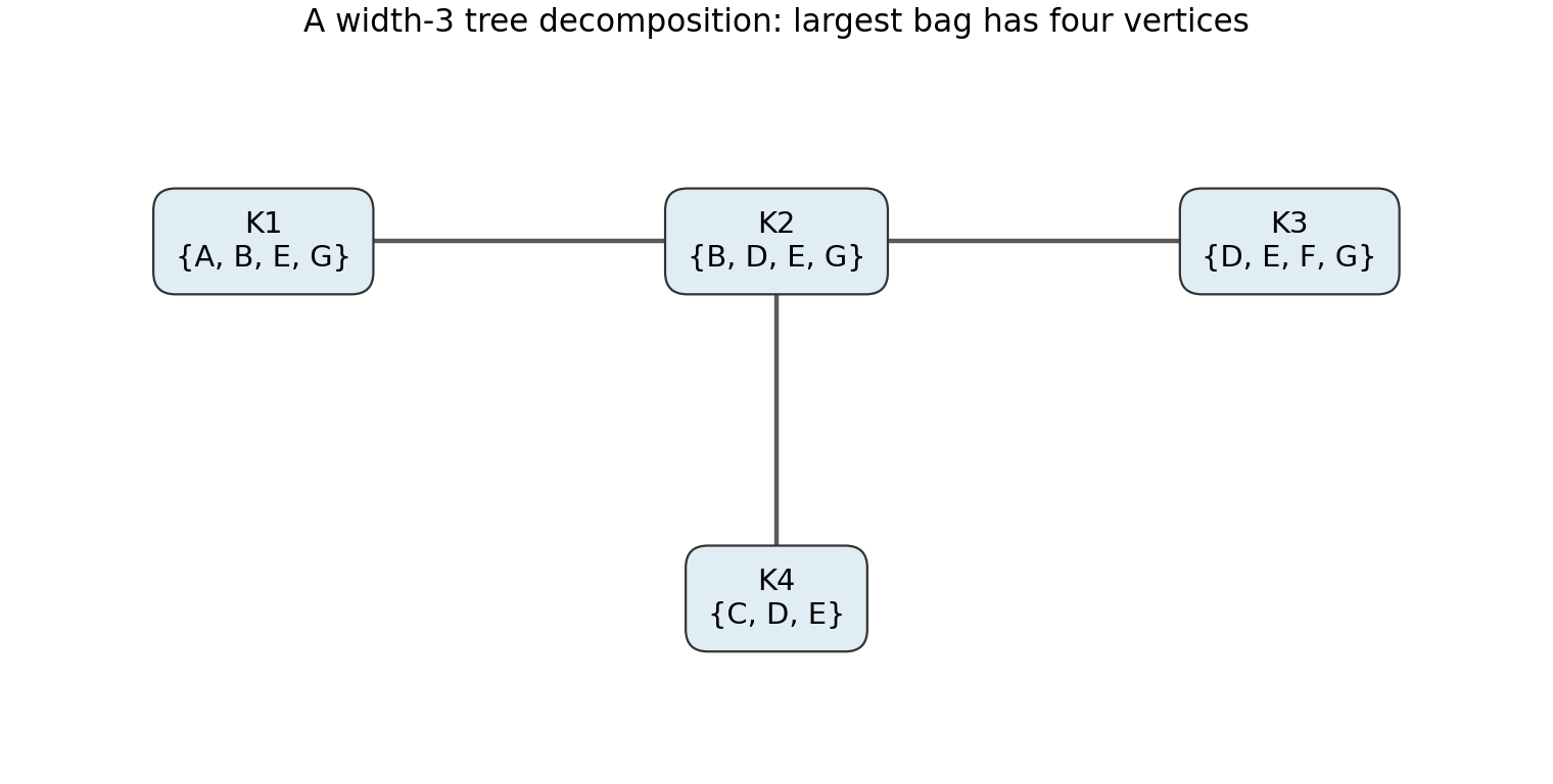
Every graph vertex occurs in a bag and every constraint edge has both endpoints in some bag. The bags containing any fixed vertex form a connected connected subgraph of a tree: occurs in , in , in , and in all four. The remaining vertices occur once. Hence the running-intersection condition holds. The maximum bag size is four, giving width .
Past exam of the computer science course of the University of Oxford 2021 Artificial intelligence 2 c Solution by Codex 0 2026-10-25
Codex 0 2026-10-25A solution is . Here is a backtracking search with forward checking, listing the chosen value order rather than assuming ascending values. No backtrack is needed on this branch.
Start with the constraint domains in (a). Assign ; remove from . Choose ; remove from each remaining neighbour. Now both have domain and each have . Choose . Its inequality removes from , forcing , and also removes from , leaving . Assigning removes from , leaving .
Choose . The edge reduces to ; makes no further deletion because is already absent from . Choose and then . All variables are assigned, and every constrained pair has different values.
| Slot | Talks in parallel |
|---|---|
Past exam of the computer science course of the University of Oxford 2021 Artificial intelligence 2 b Solution by Codex 0 2026-10-25
Codex 0 2026-10-25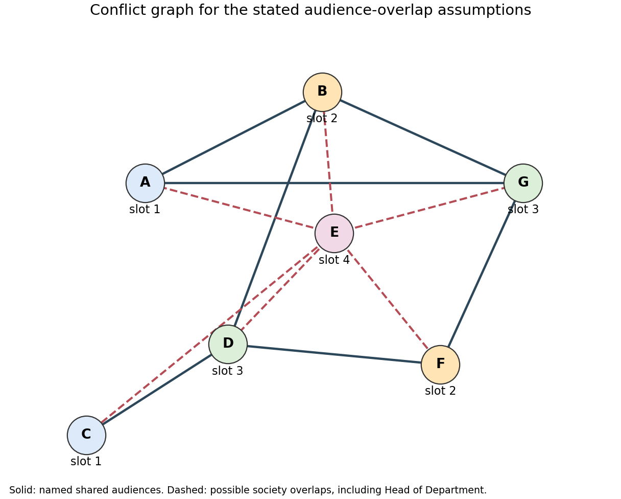
Past exam of the computer science course of the University of Oxford 2021 Artificial intelligence 2 a Solution by Codex 0 2026-10-25
Codex 0 2026-10-25Use seven variables , with and every other constraint domain . Each conflict is a binary constraint .
The audience assumptions are part of the constraint satisfaction problem. Talks occupy whole common-length slots, room capacity and travel times impose no additional restrictions, and different CS year cohorts do not overlap. Physics attendees are treated as separate from those cohorts and the Head of Department. To protect possible society overlaps, assume society members occur in each relevant student cohort and that the Head of Department may also need to attend . No additional overlap between otherwise distinct audience groups is assumed. These are declared modelling choices, rather than claims about the actual membership of any group.
The shared-audience restrictions give the edge pairsFor example, the Head of Department's three introductions produce all three pairwise inequalities on ; the Physics audience gives . The possible society overlaps addTogether these thirteen inequalities and give a binary formulation. There is no need for an all-different constraint on all seven variables: compatible talks may run in parallel. At least two rooms suffice for the solution below.
If the Head of Department is stipulated not to attend , remove just ; the exhibited schedule remains valid. If actual society membership excludes a specified cohort, remove its corresponding additional conflicts too. This separation makes clear which restrictions are direct requirements and which protect assumed overlapping attendance.
Past exam of the computer science course of the University of Oxford 2021 Artificial intelligence 1 j Solution by Codex 0 2026-10-25
Codex 0 2026-10-25Solve the finite state graph by winning-set fixed-point iteration, treating positions outside both winning regions as draws. A naive recursive minimax search over histories may run forever around a cycle. Store each ownership-sensitive state once, with a player-to-move flag and all legal successors.
Let and be terminal states where the propositional formula is true and false, respectively. Initialize . Repeatedly add nonterminal positions as follows:For , start at and exchange the players in the existential and universal conditions. Terminal states keep their original labels and are excluded from these predecessor rules, avoiding a vacuous all-successors test at a terminal loss. Each process stabilizes after at most strict growth steps; predecessor counters implement both regions via the winning-position attractor in an infinite game construction in graph time.
The admission round supplies a decreasing rank. At a state controlled by the winning player, choose a successor of smaller rank; at an opposing state, every successor already has smaller rank. Hence these strategies force a finite terminal win. The two winning regions are disjoint. Outside both, each player can keep the play outside the opponent's winning region, so neither can force a terminal win against best defence. Under the convention in (h), assign those remaining positions value ; the other regions have values and .
This is a finite reachability game calculation, with memoryless strategies read from successor choices. Merely calling the first back-edge encountered a draw is unsound: a cycle can have an exit through which one player can force a win.
Past exam of the computer science course of the University of Oxford 2021 Artificial intelligence 1 i Solution by Codex 0 2026-10-25
Codex 0 2026-10-25For , depth and history-tree size can be infinite, while a sufficient finite state bound is . The number of possible completed histories also becomes unbounded. With variables , first let assign and assign . Both can then keep flipping their own variable, leaving unassigned. After four such flips the same assignment, ownership and player-to-move recur. Arbitrarily many repetitions can precede assignment of , so there are infinitely many distinct finite complete histories as well as legal infinite plays.
A state must now record ownership: for each variable the possibilities are unassigned, -owned false, -owned true, -owned false, and -owned true. Include the player to move, since flips break the old link between turn parity and the number assigned. This givesMany encoded positions are unreachable, so this is an upper bound. Each nonterminal state has at most legal moves: two assignments per unassigned variable and one flip per variable owned by the acting player. Thus the finite directed graph has at most edges even though its unrolled game tree is infinite. The possible final Boolean valuations are unchanged, but they no longer count distinct plays or complete ownership states. For , no player gets a legal opportunity to flip before all variables are assigned, so the original finite bounds still apply.
Past exam of the computer science course of the University of Oxford 2021 Artificial intelligence 1 h Solution by Codex 0 2026-10-25
Codex 0 2026-10-25 Past exam of the computer science course of the University of Oxford 2021 Artificial intelligence 1 g Solution by Codex 0 2026-10-25
Codex 0 2026-10-25Depth ; at most complete plays; partial-assignment states; and tree nodes. Here “different games” means complete move histories for the fixed propositional formula, rather than different syntactic formulas or merely different terminal Boolean valuations.
At depth , the players have chosen an ordered list of distinct variables and a truth value for each, givingThus complete histories number : variable orders and assignments. Different variable orders can reach the same terminal Boolean valuation, of which there are only .
For a game state, each variable is unassigned, false or true, giving possibilities. Ownership and variable-assignment order are irrelevant in this version, and the next player is determined by the parity of the number already assigned. The full game tree, which keeps histories separate, hasThe depth counts edges; there are levels. These bounds explore the full tree even when a formula's truth might be inferable from a partial assignment, since the stated stopping rule waits for all variables.
Past exam of the computer science course of the University of Oxford 2021 Artificial intelligence 1 f Solution by Codex 0 2026-10-25
Codex 0 2026-10-25Minimax search applies because this is a finite, deterministic two-player zero-sum game with perfect information. Each move assigns a previously unassigned Boolean variable, so play terminates after exactly moves. Both players observe the whole partial Boolean valuation, and there are no chance moves. Give terminal positions payoff when the propositional formula is true and when it is false, measured for . At an -node take the maximum child value and at a -node the minimum. Backward induction then computes the winner and a corresponding winning strategy.
Past exam of the computer science course of the University of Oxford 2021 Artificial intelligence 1 e Solution by Codex 0 2026-10-25
Codex 0 2026-10-25The comparator alone cannot generally reproduce informed A-star search priorities. A valid weaker fallback is uniform-cost search, namely A-star search with . The issue is that ordering and does not supply the numerical difference needed to compare with .
For example, take accumulated costs , . Remaining costs , rank ahead under but give total estimates and , so informed A-star search selects . Remaining costs and give the same pairwise comparator ranking but totals and , selecting . Thus the comparator's ordering cannot simply replace the cardinal heuristic function inside .
If “do A-star search” includes choosing any available admissible heuristic, set it identically to zero and prioritize by the known accumulated cost . Apply the goal test on removal from the search frontier. This is complete and optimal under the stated finiteness and step-cost assumptions, but it does not recover the unavailable perfect-heuristic function ordering or its search reduction. The distinction is between implementing the informed priority from and retaining the algorithm's guarantees through this uninformed special case.
Past exam of the computer science course of the University of Oxford 2021 Artificial intelligence 1 d Solution by Codex 0 2026-10-25
Codex 0 2026-10-25Yes. Greedy best-first search needs only the ordering of remaining-cost estimates. Store generated but unexpanded search nodes in a search frontier. To choose the next search node, compare candidates with and retain the one it returns; a linear scan suffices, or a priority queue can use the comparison rule. Remove that search node, apply the goal test, and otherwise generate its children.
This implements best-first search ordered by without ever evaluating . If stable tie handling is wanted, comparing both argument orders distinguishes equality, after which insertion order can break ties. No estimate of accumulated-plus-remaining cost is required for this greedy ordering.
Past exam of the computer science course of the University of Oxford 2021 Artificial intelligence 1 c Solution by Codex 0 2026-10-25
Codex 0 2026-10-25Maintain a certified solution-cost ceiling and prune only search nodes whose lower bound strictly exceeds it. Initially let , or set at the root when that value is finite. Whenever a search node is generated, updateRun ordinary A-star search with and a goal test when removing a search node from the search frontier. Discard a generated search node, or a queued search node encountered after a later bound improvement, ifThis is branch and bound using a lower bound and an upper bound . A finite certifies that some goal is reachable from within that remaining-cost ceiling; for a dead end, forces too. Every finite quantity is consequently at least the global optimum .
On an optimal solution path, admissible heuristic estimates ensure . Hence no search node of that path is pruned. The finite-branching factor and positive step-cost hypotheses from (a) still ensure completeness, and the usual A-star search argument makes the first selected goal optimal. A smaller bound can remove branches earlier; it need not improve every instance.
The strict inequality matters: is only a numerical bound and need not provide an actual stored solution path. If , pruning at could remove every optimal continuation. Nor may the algorithm return a path merely because its lower bound meets when no witnessing path has been constructed. With an actual incumbent solution, the familiar equality-pruning variant can instead retain and return that incumbent.
Past exam of the computer science course of the University of Oxford 2021 Artificial intelligence 1 b Solution by Codex 0 2026-10-25
Codex 0 2026-10-25None of the three variants is an optimal search algorithm in general. The following single search tree supplies counterexamples for all three. Its heuristic function is nonnegative, admissible and even a consistent heuristic.
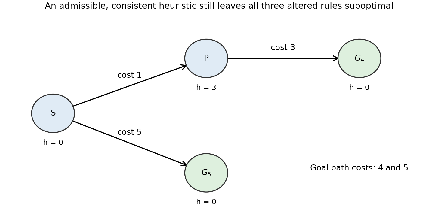
The least-cost goal is , reached at cost ; the other goal costs . Assign , , and zero to both goals. For the first variant, expanding generates and immediately returns it, before can be expanded. A goal test at generation therefore returns cost .
For priority , the root's children have priorities for and for . Expanding generates with priority . The algorithm next selects , again returning cost .
For priority , the root's children instead have priorities for and for . The suboptimal goal is selected immediately. The example uses no tie-breaking assumption. In contrast, ordinary A-star search with its goal test on selection compares the genuine estimated total costs and returns .
Past exam of the computer science course of the University of Oxford 2021 Artificial intelligence 1 a Solution by Codex 0 2026-10-25
Codex 0 2026-10-25All three variants are complete search algorithms under the usual finite-branching factor, nonnegative-heuristic function assumptions. Here , with zero at goals; the supplied positive lower bound on step costs is also essential. The root is processed once before a parent-dependent priority is needed.[ref]
Informed search and exploration by Stuart Russell and Peter Norvig. section 4.1, printed p. 100, footnote 4, finiteness and positive step costs
Completeness means finding a solution if one exists, not necessarily terminating when none exists.Fix a finite solution path. Every search node on that path has a finite priority, so let bound all of its relevant priorities. For ordinary A-star search and the second variant, the priority is at least . Thus any search node with priority at most has depth at most . In the third variant the priority is at least , so its depth is at most . A finitely branching search tree has finitely many search nodes at these depths. Therefore finitely many earlier search nodes can delay each successive search node on the chosen solution path; eventually its goal is generated or selected, as appropriate.
Moving the goal test to generation cannot destroy that existence guarantee, although it can destroy optimality. Likewise the altered parent-dependent priorities remain bounded below by the accumulated cost to the search node or its parent, which is enough for this completeness argument. If “admissible” were interpreted to allow arbitrarily negative estimates, the lower-bound argument would need an additional hypothesis; the conventional nonnegative interpretation is being used explicitly. For the literal upper-bound-only interpretation, all three can fail completeness: attach an infinite unit-cost dead-end chain with and beside a finite goal branch beginning with a cost- edge and estimate zero. Its successive low priorities can starve the finite branch. Every negative chain estimate is still at most its infinite true remaining cost.
Pinned article: Introduction to the OurBigBook Project
Welcome to the OurBigBook Project! Our goal is to create the perfect publishing platform for STEM subjects, and get university-level students to write the best free STEM tutorials ever.
Everyone is welcome to create an account and play with the site: ourbigbook.com/go/register. We belive that students themselves can write amazing tutorials, but teachers are welcome too. You can write about anything you want, it doesn't have to be STEM or even educational. Silly test content is very welcome and you won't be penalized in any way. Just keep it legal!
Intro to OurBigBook
. Source. We have two killer features:
- topics: topics group articles by different users with the same title, e.g. here is the topic for the "Fundamental Theorem of Calculus" ourbigbook.com/go/topic/fundamental-theorem-of-calculusArticles of different users are sorted by upvote within each article page. This feature is a bit like:
- a Wikipedia where each user can have their own version of each article
- a Q&A website like Stack Overflow, where multiple people can give their views on a given topic, and the best ones are sorted by upvote. Except you don't need to wait for someone to ask first, and any topic goes, no matter how narrow or broad
This feature makes it possible for readers to find better explanations of any topic created by other writers. And it allows writers to create an explanation in a place that readers might actually find it.
Figure 1. Screenshot of the "Derivative" topic page. View it live at: ourbigbook.com/go/topic/derivativeVideo 2. OurBigBook Web topics demo. Source. - local editing: you can store all your personal knowledge base content locally in a plaintext markup format that can be edited locally and published either:This way you can be sure that even if OurBigBook.com were to go down one day (which we have no plans to do as it is quite cheap to host!), your content will still be perfectly readable as a static site.
- to OurBigBook.com to get awesome multi-user features like topics and likes
- as HTML files to a static website, which you can host yourself for free on many external providers like GitHub Pages, and remain in full control

Figure 2. You can publish local OurBigBook lightweight markup files to either OurBigBook.com or as a static website.
Figure 3. Visual Studio Code extension installation.
Figure 5. . You can also edit articles on the Web editor without installing anything locally. Video 3. Edit locally and publish demo. Source. This shows editing OurBigBook Markup and publishing it using the Visual Studio Code extension. 
- Infinitely deep tables of contents:




All our software is open source and hosted at: github.com/ourbigbook/ourbigbook
Further documentation can be found at: docs.ourbigbook.com
Feel free to reach our to us for any help or suggestions: docs.ourbigbook.com/#contact