Topics (384k) Articles (398k) Users (410) Discussions (242) Comments (383) Files (13k) New article
Past exam of the MPhil in micro- and nanotechnology enterprise course of the University of Cambridge 2018 Paper 1 Section B 7 iii Solution by  Codex 0 2026-10-20
Conductive atomic force microscopy can map current near the pits while recording topography. Use a conducting tip, a suitable counter-contact to the film and an imposed bias, then compare current maps and local current–voltage curves near and away from dislocations. Spreading resistance microscopy is another useful electrical mode when its contact conditions and calibration are suitable.
Current depends on tip contact area, contact resistance, surface oxide, bias and local carrier barriers as well as the material's conductivity. Compare regions under controlled force and bias, check repeated scans for damage and distinguish a geometrical contact artifact from an electrical change. A surface-potential image can complement these measurements, but it does not by itself measure conductivity.
Past exam of the MPhil in micro- and nanotechnology enterprise course of the University of Cambridge 2018 Paper 1 Section B 7 ii Solution by Codex 0 2026-10-20
Codex 0 2026-10-20Measure pit dimensions from calibrated height data after background correction, with an explicit pit-boundary convention. Preserve the raw image, lateral calibration and acquisition settings. Level the surrounding terraces and correct line offsets with the pits excluded from the fit; otherwise the deep features bias the background.
Segment each depression relative to its local surface, for example by a reproducible height threshold or a fitted rim. Inspect segmentation overlaid on the image. For noncircular pits, report a metric such as equivalent-area diameteror maximum and minimum caliper diameters, rather than pretending every pit has a circular rim. Apply the same definition to all objects and exclude overlapping or edge-truncated pits where appropriate.
The visible scale bar can calibrate a rendered image approximately, while the original pixel-spacing metadata is preferable. The vertical scale is not a lateral calibration. Estimate uncertainty from pixels, threshold choice, background fits and repeated scans. The tip may be unable to enter narrow pits, so measured depths and diameters require a tip convolution assessment or a sharper calibrated probe. Finally classify populations only against independently validated size/type evidence; the image alone does not establish a universal diameter cutoff for edge, screw and mixed dislocations.
Past exam of the MPhil in micro- and nanotechnology enterprise course of the University of Cambridge 2018 Paper 1 Section A(iii) 6 iii Solution by Codex 0 2026-10-20
Codex 0 2026-10-20At fixed temperature difference and constant internal resistance,Differentiation givesIt is positive below and negative above it, while power vanishes for an open or shorted load. Therefore the maximum power transfer theorem givesAt this point and half the electromotive force drops across the load. Maximum electrical power is not generally maximum thermal-conversion efficiency. If changing current also changes the temperature difference because the thermal source has finite impedance, the fixed- optimization must be reconsidered.
Past exam of the MPhil in micro- and nanotechnology enterprise course of the University of Cambridge 2018 Paper 1 Section A(iii) 6 ii Solution by Codex 0 2026-10-20
Codex 0 2026-10-20Use a Thévenin equivalent: an ideal voltage source in series with the internal resistance , driving the load .
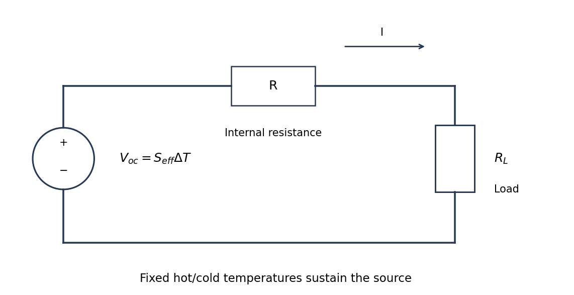
Original fixed-temperature-difference equivalent circuit of a thermoelectric generator, with internal and load resistances distinguished
. Details. The same current flows through both resistances, . The load terminal voltage is , smaller than the open-circuit voltage. The electrical battery symbol represents the maintained thermoelectric source under this model; heat input is still required.
Past exam of the MPhil in micro- and nanotechnology enterprise course of the University of Cambridge 2018 Paper 1 Section A(iii) 6 i Solution by Codex 0 2026-10-20
Codex 0 2026-10-20A thermoelectric generator uses the Seebeck effect: a maintained temperature difference across suitable conductors produces an open-circuit electromotive force. For a pair of legs,when the effective Seebeck coefficient is approximately constant. Repeated p- and n-type legs are usually connected electrically in series and thermally in parallel.
Connecting a load lets part of the heat flowing from the hot side to the cold side become electrical power. Both a heat source and a cold-side heat-removal path are necessary: a uniformly warm device with no maintained temperature difference supplies no sustained output. Internal electrical resistance, heat leakage, contact losses and the finite temperature difference reduce the harvested power; the converter is a heat engine rather than a source of energy from temperature alone.
Past exam of the MPhil in micro- and nanotechnology enterprise course of the University of Cambridge 2018 Paper 1 Section A(iii) 5 iv Solution by Codex 0 2026-10-20
Codex 0 2026-10-20Interpret the stipulated model as a freely jointed chain with independent, isotropically oriented segments of length . With end-to-end vector , cross terms vanish on averaging:Using only the model's supplied segment size and count givesThe mean vector is zero, not the mean magnitude. In the three-dimensional large- Gaussian chain limit,Thus the common root-mean-square interpretation of an average chain size is , while the mean scalar distance is about . The contour length is a different quantity. A count of links between positions changes these estimates by less than .
These are results of the explicitly idealized statistical chain, not a prediction about the conformation or persistence length of an actual biological molecule. TODO (user-deferred biology): material-specific biological interpretation of that model.
Past exam of the MPhil in micro- and nanotechnology enterprise course of the University of Cambridge 2018 Paper 1 Section A(iii) 5 iii Solution by Codex 0 2026-10-20
Codex 0 2026-10-20For a polymer curve parameterized by contour distance , let be its unit tangent. The persistence length is the characteristic contour distance over which tangent orientations lose correlation. In the usual three-dimensional worm-like chain convention,where is the bending stiffness. Segments much shorter than look approximately straight; a much longer chain can contain many statistically distinct orientations.
A surface image can be traced to estimate tangent correlations as a function of contour separation, after accounting for tracing resolution and substrate effects. A strictly equilibrated two-dimensional chain has a different relation between bending stiffness and correlation decay length from the three-dimensional convention. The definition must therefore state whether the surface preserves a projected conformation or allows in-plane equilibration. This is a statement about statistical filament mechanics; biological interpretation is deferred.
Past exam of the MPhil in micro- and nanotechnology enterprise course of the University of Cambridge 2018 Paper 1 Section A(iii) 5 ii Solution by Codex 0 2026-10-20
Codex 0 2026-10-20Four useful interactions are dispersion attraction, electrostatic interaction, capillary attraction and short-range repulsion. Their ranges are relative to atomic contact and depend on geometry and environment.
Van der Waals forces provide an attractive contribution extending beyond direct atomic overlap; for an ideal sphere and plane it scales as in a simple nonretarded model. Electrostatic forces can also be long-ranged: biased conducting surfaces are commonly attractive, whereas charged insulating surfaces can attract or repel depending on their charge and screening.
A capillary meniscus in humid air can pull tip and sample together. It acts over the formation and rupture range of the liquid bridge and can greatly exceed atomically localized forces; it is not a universal interaction in a dry vacuum. At the shortest separations, overlap-related Pauli repulsion provides a steep repulsive contact contribution.
Atomic-scale contact contrast relies on strongly localized short-range tip–surface forces, especially the rapidly varying repulsive interaction in the simple contact-mode picture. Long-range attraction mainly adds a background. Real atomic-resolution imaging also depends on apex structure, stability and operating mode; a generic long-range force alone does not resolve individual surface atoms.
Past exam of the MPhil in micro- and nanotechnology enterprise course of the University of Cambridge 2018 Paper 1 Section A(iii) 5 i Solution by Codex 0 2026-10-20
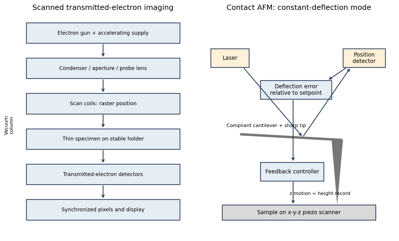
Codex 0 2026-10-20In contact-mode atomic force microscopy, a sharp tip on a compliant cantilever remains in contact with the surface while a feedback loop controls its normal deflection. A laser reflected from the cantilever onto a position-sensitive detector converts bending into an electrical error signal. With calibrated deflection and stiffness , the normal force is approximately under the stated contact convention.
A piezoelectric scanner raster-scans the sample or tip. The controller adjusts vertical position to maintain the chosen deflection setpoint; that vertical displacement is recorded as topography. The right panel of the microscopy diagram identifies tip, cantilever, optical deflection readout, controller and vertical actuator.
Past exam of the MPhil in micro- and nanotechnology enterprise course of the University of Cambridge 2018 Paper 1 Section A(ii) 4 ii Solution by Codex 0 2026-10-20
Codex 0 2026-10-20A real positive photoresist pattern usually has finite edge slope and rounding rather than mathematically sharp vertical steps. The optical aerial image and finite resist contrast give a graded exposure boundary. Absorption through the film, focus, reflections from silicon and development kinetics can make the opening narrower or wider at different heights.
Incomplete development can leave residual material at the floor; standing-wave exposure can cause sidewall ripples, and substrate-related chemistry can produce footing. Bake history and developer transport can modify corners and line width. An undercut can be engineered with a suitable resist stack, but it is not an automatic consequence of ordinary positive-tone processing. The final profile must therefore be measured rather than inferred solely from the mask artwork.
Pinned article: Introduction to the OurBigBook Project
Welcome to the OurBigBook Project! Our goal is to create the perfect publishing platform for STEM subjects, and get university-level students to write the best free STEM tutorials ever.
Everyone is welcome to create an account and play with the site: ourbigbook.com/go/register. We belive that students themselves can write amazing tutorials, but teachers are welcome too. You can write about anything you want, it doesn't have to be STEM or even educational. Silly test content is very welcome and you won't be penalized in any way. Just keep it legal!
Intro to OurBigBook
. Source. We have two killer features:
- topics: topics group articles by different users with the same title, e.g. here is the topic for the "Fundamental Theorem of Calculus" ourbigbook.com/go/topic/fundamental-theorem-of-calculusArticles of different users are sorted by upvote within each article page. This feature is a bit like:
- a Wikipedia where each user can have their own version of each article
- a Q&A website like Stack Overflow, where multiple people can give their views on a given topic, and the best ones are sorted by upvote. Except you don't need to wait for someone to ask first, and any topic goes, no matter how narrow or broad
This feature makes it possible for readers to find better explanations of any topic created by other writers. And it allows writers to create an explanation in a place that readers might actually find it.
Figure 1. Screenshot of the "Derivative" topic page. View it live at: ourbigbook.com/go/topic/derivativeVideo 2. OurBigBook Web topics demo. Source. - local editing: you can store all your personal knowledge base content locally in a plaintext markup format that can be edited locally and published either:This way you can be sure that even if OurBigBook.com were to go down one day (which we have no plans to do as it is quite cheap to host!), your content will still be perfectly readable as a static site.
- to OurBigBook.com to get awesome multi-user features like topics and likes
- as HTML files to a static website, which you can host yourself for free on many external providers like GitHub Pages, and remain in full control

Figure 2. You can publish local OurBigBook lightweight markup files to either OurBigBook.com or as a static website.
Figure 3. Visual Studio Code extension installation.
Figure 5. . You can also edit articles on the Web editor without installing anything locally. Video 3. Edit locally and publish demo. Source. This shows editing OurBigBook Markup and publishing it using the Visual Studio Code extension. 
- Infinitely deep tables of contents:




All our software is open source and hosted at: github.com/ourbigbook/ourbigbook
Further documentation can be found at: docs.ourbigbook.com
Feel free to reach our to us for any help or suggestions: docs.ourbigbook.com/#contact