In the high-surface-potential Schulze-Hardy rule, the critical coagulation concentration scales approximately as $z^{-6}$ with the counterion valence. HenceThe more highly charged counterion therefore requires about eleven times less concentration in this idealized estimate. This assumes the cations are the counterions of a negatively charged surface, the surface-potential regime is appropriate, and the only changing mechanism is electrostatic stabilization. Specific adsorption and hydrolysis of aluminium ions can invalidate this scaling; matching ionic strengths instead is not the same prediction.

charge stabilization of colloids supplies repulsion when like-charged surfaces and their electric double layers approach. steric stabilization uses attached or adsorbed molecular layers whose overlap costs conformational and osmotic free energy. Combining both gives electrosteric stabilization; a solvated coating must remain attached and well solvated. A viscous medium slows encounters but does not by itself create an equilibrium repulsive barrier.

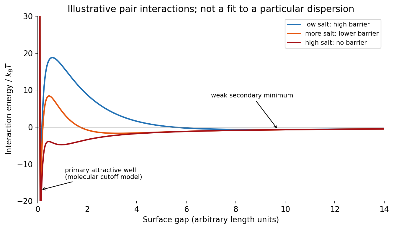
DLVO theory adds screened electrostatic repulsion to Van der Waals force. A representative close-gap form isfor equal spheres of radius $a$, with Hamaker constant $A_H$ and inverse Debye–Hückel screening length $\kappa$. The formula is schematic near molecular contact, where hydration, surface roughness and finite ion size matter. A repulsive barrier many $k_{B}T$ high produces kinetic stability even if the primary attractive minimum is deeper than the dispersed state. Entry into that primary minimum generally gives strongly bound aggregation; a shallow secondary minimum can give reversible flocculation.

Adding electrolyte increases $\kappa$, shortens the repulsion and can remove the barrier, enabling fast diffusion-limited aggregation. The critical coagulation concentration is the approximate salt concentration at which this rapid-coagulation regime begins under specified conditions. It is not a universal property of the salt alone. Test the prediction using time-resolved dynamic light scattering or turbidity at controlled particle concentration, pH and temperature; check that added ions do not specifically adsorb or change the surface chemistry.

First, use a phase-shift mask: neighbouring openings transmit appropriately phased light, increasing the intensity slope and improving separation of neighbouring bright regions. The benefit is pattern dependent and phase conflicts or mask defects must be controlled. Second, use off-axis illumination matched to the grating orientation, so useful diffracted orders fall inside the projection pupil and contribute interference contrast at smaller pitch. Check orientation dependence and the reduced process window; it does not enlarge the geometrical pupil.

Third, use optical proximity correction and subresolution assist features to compensate the pattern-dependent aerial-image distortion at edges and corners. Verify the printed critical dimensions using a focus–exposure matrix and scanning electron microscopy. These are three adaptations of the existing exposure process that lower effective $k_1$; none promises arbitrary subwavelength structure. A thinner, higher-contrast photoresist and an antireflection underlayer can further improve pattern transfer, but do not change the wavelength.

An immersion liquid increases numerical aperture through $NA=n\sin \alpha$, if the optics can use the same ray angle $\alpha$ inside a transparent, chemically compatible liquid of refractive index $n$. With unchanged $k_1$ and vacuum wavelength, the width scales as $R_{\mathrm{imm}}=R_{\mathrm{air}}/n$ at fixed angle. If the two empirical formulae printed in the question are used literally with fixed $k_2$, they give $DO{F}_{\mathrm{imm}}=300/n^2\mathrm{nm}$.

For a physical axial displacement inside the medium, however, the familiar paraxial defocus range contains an additional index factor: $DOF\propto n{\lambda }_0/N{A}^2$. That convention gives $DO{F}_{\mathrm{imm}}/DO{F}_{\mathrm{air}}\simeq 1/n$ at fixed ray angle, or an approximately $n$-fold larger depth of focus at fixed $NA$ and resolution. Thus immersion can improve lateral resolution, while its focus benefit depends on what is held fixed and on the axial-focus convention. It cannot improve resolution merely by inserting $n$ into $NA$ while ignoring optical redesign, absorption or resist compatibility. No liquid index is supplied for a numerical prediction.

Solve the stated depth of focus relation before substituting into the resolution expression:This uses the supplied empirical $k_1$ and $k_2$ unchanged and interprets $R$ as the minimum line or space width of an equal-line/space square grating. Under that convention its pitch is $2R=578.6\mathrm{nm}$. Other pattern shapes or a different definition of the quoted depth of focus would require different process factors.

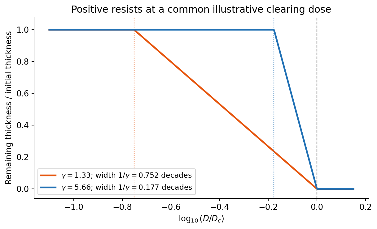
On a graph of normalized remaining thickness against ${\log }_{10}D$, both positive photoresist curves remain near unity below $D_0$ and fall to zero by $D_c$. Their transition widths are ${\log }_{10}(D_c/D_0)=1/\gamma$: $0.752$ decades for the lower-contrast material and $0.177$ decades for the higher-contrast material. The latter therefore has a much steeper transition. The curves can be aligned at a common illustrative clearing dose; their absolute horizontal placement cannot be inferred from photoresist contrast alone.

The higher-contrast material distinguishes bright and dark regions even when diffraction has reduced their intensity modulation. The lower-contrast material requires a much stronger aerial-image modulation and loses small features earlier. Finite resist thickness, standing waves, acid diffusion, development conditions and photon statistics can limit actual performance beyond this threshold model.

For a positive photoresist, let $D_0$ be the largest exposure preserving the initial film thickness and $D_c$ the clearing dose. The photoresist contrast is $\gamma =1/{\log }_{10}(D_c/D_0)$. An aerial image $I=\bar{I}[1+M\cos (2\pi \nu x)]$ can clear its maxima while retaining its minima only ifThus $M_c=0.6991$ and $0.2006$ for the lower- and higher-contrast materials. Reading those levels on the supplied modulation transfer function gives maximum normalized spatial frequencies approximately $\nu /{\nu }_0=0.40$ and $0.60$, respectively. The stated partial coherence is already represented by that curve; do not multiply the read frequencies by another coherence factor.

The unambiguous pattern dimensions are full pitch $P=1/(x{\nu }_0)$ and equal line/space width $w=P/2$, where $x$ is the read normalized frequency. To convert the paper's Rayleigh-frequency label into lengths, explicitly use the circular-pupil Rayleigh criterion $d_R=0.61\lambda /NA$ and ${\nu }_0=1/d_R$. With the ArF vacuum wavelength $193\mathrm{nm}$ and the stated numerical aperture, $d_R=235.5\mathrm{nm}$, givingThe higher-contrast material resolves a line/space feature about two-thirds as wide. The pitch and half-pitch distinction matters: the point-separation Rayleigh criterion is not itself an equal-line/space width. If a course defines ${\nu }_0$ as an optical cutoff rather than $1/d_R$, use that specified frequency in $w=1/(2x{\nu }_0)$; the normalized graph readings and their ratio are unchanged. No absolute clearing dose is provided.

Three suitable approaches give complementary contrast. tapping-mode atomic force microscopy supplies surface topography and an oscillation-phase image. It reduces lateral drag and is often effective for soft block copolymer domains. Its phase contrast depends on elastic response, adhesion, dissipation and operating setpoint together: a bright phase domain is not automatically the stiffer polymer. Check contrast as amplitude and setpoint change and use a known reference.

quantitative nanomechanical mapping fits the repulsive portions of many AFM force curves and separately maps effective elastic modulus, adhesion and deformation. It directly addresses the stiffness difference and limits maximum force. Its quantitative result depends on tip radius, force calibration, contact model, loading rate and film thickness; domains narrower than the contact footprint are mixed and the substrate can dominate a thin film. Use small indentation, substrate controls and a suitable viscoelastic interpretation.

friction force microscopy can reveal domains with different frictional and adhesive response, using torsional deflection during contact scans. It is simple and sensitive to surface chemistry, but continuous shear may deform or displace soft domains, and slope/topography can contaminate the lateral signal. Acquire trace–retrace pairs at several low normal loads and check reproducibility. Use a mechanical-modulus map to test the stiffness assignment; phase or friction contrast alone does not uniquely identify stiffness or chemical composition.

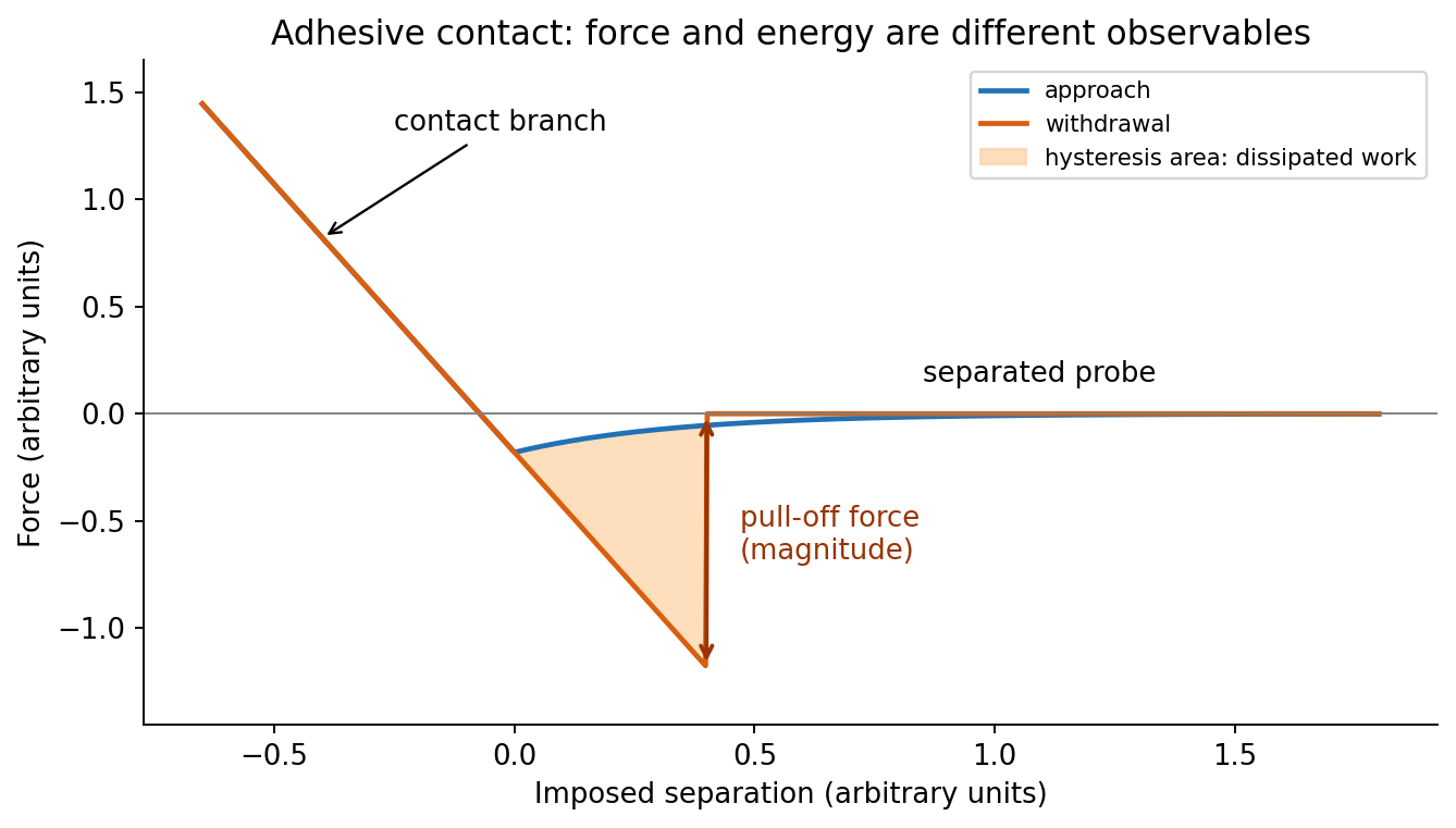
In quantitative nanomechanical mapping, the operational adhesion is the magnitude of the most attractive force immediately before detachment on a calibrated retraction curve:Here $k_c$ is the cantilever spring constant and ${\delta }_c$ its deflection after baseline subtraction. The area between approach and retraction relates to dissipated work, whereas the minimum force is a force, not an energy. Chemical attraction, Van der Waals forces and ambient-water capillary bridges can all contribute. Match loading rate and peak load, calibrate deflection sensitivity and $k_c$, compare clean reference surfaces, and control humidity; otherwise different maps may reflect different tips or capillary conditions rather than different specimens.

At position (1), the AFM probe is far from the surface, with approximately zero force. At (2), attractive interactions bend the AFM cantilever toward the surface; when the attractive force gradient exceeds the cantilever spring constant, the equilibrium becomes unstable and jump-to-contact occurs. Position (3) is on the mechanical-contact branch: changes in imposed height largely bend the AFM cantilever and, for a compliant specimen, indent the sample. This branch can include compressive contact and adhesive contact under tension; contact does not itself imply a positive force at every point. At (4), during withdrawal the tip remains attached and pulls the AFM cantilever downward until the pull-off force is reached and it detaches. Approach and retraction follow different paths because adhesion creates a hysteretic contact. The numbered points identify stages on the source curve, not four extra question parts.

piezoelectric scanner creep is the continued slow displacement after a step in scanner drive, even when the commanded voltage has stopped changing. The scanner's strain continues to relax, and the motion can resemble a slowly decaying, approximately logarithmic drift. After changing scan size, position or offset, early lines can therefore have stretched or compressed coordinates. Allow settling, avoid large abrupt moves, use a position-sensor closed-loop control system, and compare repeated images. This time-dependent response differs from the direction-dependent piezoelectric hysteresis and from ordinary thermal drift.

The repeated, similarly oriented rounded triangular outlines in panel (a) are characteristic of AFM tip convolution: a narrow raised object can image the shape of a blunt or contaminated AFM probe, rather than reveal its own lateral shape. A finite tip radius broadens lateral dimensions. Replace or clean the AFM probe, check it on an independently characterized sharp-feature standard, and repeat at low load; agreement after a tip change is stronger evidence than a visually pleasing image. Image processing cannot uniquely recover unmeasured sidewalls or prove that every particle with a similar outline is an artefact.

Panel (b) contains horizontal streaks associated with steep features. The natural instrumental diagnosis is AFM feedback artefact: the height controller does not track a rapid change faithfully, or rings after it. Reduce the scan speed and adjust proportional/integral gains below the oscillation threshold. Compare trace and retrace and rotate the fast-scan direction: a streak following the scan rather than the specimen is instrumental. Loose contamination can also produce scan-line streaks, so clean or change the AFM probe if tuning does not remove them. Tip-shape broadening in (a), and scan-direction tracking/streaking in (b), are the principal diagnoses; the images alone do not uniquely establish every underlying cause.

For $\omega \tau \ll 1$,andThus the material flows at sufficiently low frequency: its static shear modulus vanishes and its terminal response is viscous. The dashpot in the Maxwell branch allows its spring stress to relax, so there is no permanent elastic path through the parallel network.

The fact that both $G^{\prime }$ and $G^{\prime \prime }$ tend to zero is not evidence of a force-free material: stress at fixed shear rate tends to ${\eta }_0\dot{\gamma }$. At higher frequency the spring stores energy, but a finite-frequency elastic response does not make the long-time material a solid.

Let the Maxwell branch contain spring modulus $G$ and series viscosity ${\eta }_M$, in parallel with a dashpot of viscosity ${\eta }_s$. The branch strains are equal and stresses add. Writing ${\sigma }_M$ for the Maxwell stress,For $\gamma =\mathrm{Re}({\gamma }_0{e}^{i\omega t})$ and $\tau ={\eta }_M/G$,Multiplying the Maxwell fraction by $1-i\omega \tau$ givesThe sign of the imaginary coefficient depends on the phasor convention; these expressions use $e^{i\omega t}$, so $G^{\prime \prime }>0$ represents dissipation. In the time domain, the equivalent constitutive relation isThe original mechanical schematic shows the series spring/dashpot branch separately from the parallel dashpot.