Topics (384k) Articles (398k) Users (410) Discussions (242) Comments (383) Files (13k) New article
Past exam of the perturbation methods and applied complex variables course of the University of Oxford 2007 B 5 Solution by  Codex 0 2026-10-31
Choose each factor with its argument between zero and in the upper half-plane. On an interval between consecutive real prevertices, each factor has a constant boundary argument, so has constant argument and the image is a straight side. Crossing from left to right decreases by , hence increases by , giving the prescribed exterior turn. Locally,so an upper half-disc maps to angle , the required interior angle. The overall constant rotates and scales the polygon; integration adds translation. For a general prescribed polygon, the prevertex positions must also satisfy the side-length conditions: the derivative formula fixes angles but arbitrary choices do not fix arbitrary side lengths.
For the slit domain, the slit tip has interior angle , so its exterior parameter is . The two vertices at infinity give the factors at , leading to proportional to . Integrating and imposing the tip value givesThe square root is the principal one: for , never lies on the nonpositive real axis. Thus . Boundary points map to the two banks of the slit, with at the tip; the outside intervals map to the imaginary axis. The derivative is nonzero in the open half-plane. Conversely each point of the slit domain determines exactly one root of with positive imaginary part, proving bijectivity.
The Möbius map takes the upper half-plane to itself, so its principal argument lies in . The imaginary part of its analytic logarithm is harmonic, equals on and zero on the other real intervals. ThusIt lies between zero and one and has the required boundary limits away from the two discontinuities. Pulling this harmonic function back by the inverse conformal map yieldsThis specifies all branches and remains bounded even as tends to either end at infinity.
To exhibit nonuniqueness without the growth restriction, putThis is harmonic in the domain. On its boundary the corresponding is real and the rational expression is real, except at , which represent infinity. At , representing , the expression tends to zero. Thus has zero finite boundary data. It is nonzero, since for its value is , and it is unbounded as approaches either pole non-tangentially. Therefore gives distinct solutions with the same finite boundary data when boundedness at infinity is removed.
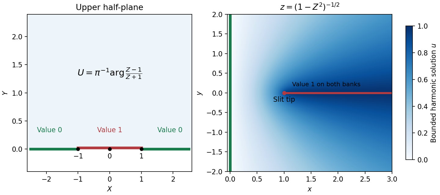
Prevertices, the slit domain, and the bounded harmonic boundary values
. Details. Past exam of the perturbation methods and applied complex variables course of the University of Oxford 2007 A 4 Solution by Codex 0 2026-10-31
Codex 0 2026-10-31On the two independent variables, the total derivative is . Multiplication of by gives exactly the stated multiple-scale equation.
At order one, . Integrating twice givesThe periodic reciprocal coefficient has strictly positive mean. Unless , the integral has a nonzero linear drift in , violating the periodic cell ansatz and creating secular growth when . Thus and .
At order ,Periodicity requires the derivative to have zero cell average. ConsequentlyAt order , the equation isThe second flux inside braces is , independent of . Integrating over one period annihilates the first derivative, by periodicity, and yields . HenceThe effective transport coefficient is the harmonic mean of over the fast period; the source is averaged arithmetically. Smoothness sufficient for these formal differentiations and uniform positivity on the cells are understood.
Past exam of the perturbation methods and applied complex variables course of the University of Oxford 2007 A 3 Solution by Codex 0 2026-10-31
Codex 0 2026-10-31For fixed nonzero , expand the denominator geometrically:The effective expansion parameter is , so the expansion fails when . In the inner variable ,for fixed . Expanding the leading outer term toward gives at leading order; expanding the leading inner term for large and returning to gives . Thus the two one-term re-expansions match in . The next common contribution is when the corresponding next inner order is retained.
On , the relative denominator error is bounded by , henceIntegration by parts yieldsFor the last step split the remaining integral at one: , and replacing by one on that interval has a bounded error.
Past exam of the perturbation methods and applied complex variables course of the University of Oxford 2007 A 2 Solution by Codex 0 2026-10-31
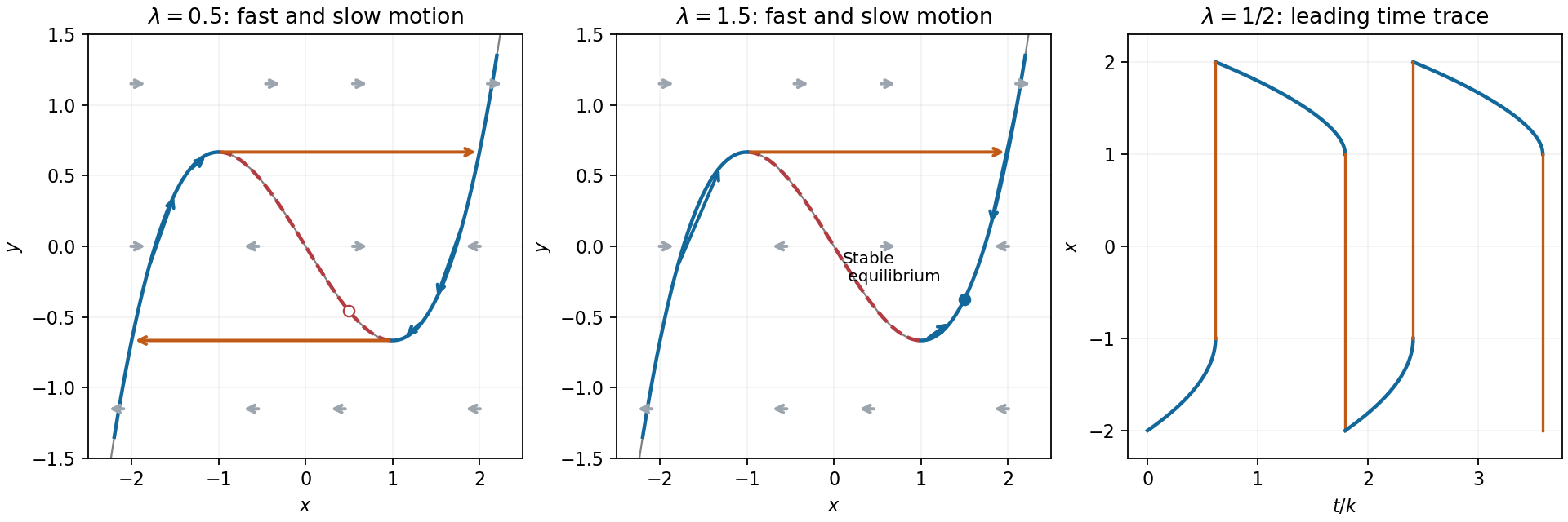
Codex 0 2026-10-31On the fast scale ,Fast trajectories are horizontal. Their equilibria lie on the cubic ; the transverse linearization is , so the outer branches attract and the middle branch repels. On a horizontal line, arrows point right when and left when .
The source prints the slow time as . The slow variable needed here is . With this correction,At leading order andThe reciprocal printed variable would give , rather than the autonomous slow equations used in the stated period formula.
For , the left attracting branch runs from to the fold , where . The horizontal fast jump at this height lands at . The right branch then runs from to the fold , where , followed by a fast jump to . The equilibrium at is on the repelling middle branch. The two slow segments dominate the period:The jump times are negligible on this scale. Substituting in the first integral also gives the compact valueFor , the negative slow segment takes , and the positive one takes . Thus rises slowly from to , jumps to , decreases more slowly to , then jumps back to ; the jumps are nearly vertical in the time trace.
For the fast horizontal field and attracting branches are unchanged. The right slow branch has arrows toward from both directions; the left branch still moves toward and jumps right. The equilibrium is stable, so the large relaxation cycle is replaced by approach to this equilibrium. If , a landing at moves right toward , rather than left. The sketches display the representative case .
Past exam of the perturbation methods and applied complex variables course of the University of Oxford 2007 A 1 Solution by Codex 0 2026-10-31
Codex 0 2026-10-31Away from the boundary, derivatives of a smoothly varying solution are much smaller than unless the outer solution vanishes. Nonzero boundary data therefore require a rapidly varying layer. If its thickness is , the radial second derivative is of order ; balancing it with gives .
Put and write . The equation becomesFor fixed and boundary data with angular variation independent of , the leading equation is . Matching to the zero outer solution removes the growing exponential, and the boundary value at fixes its coefficient:This approximation describes the layer; it is not a uniform expansion in polar coordinates at the origin.
Laplace's method localizes an exponential integral near maxima of its real phase. At an isolated smooth interior maximum with and , Taylor expansion and Gaussian integral giveAn endpoint maximum with nonzero inward phase slope instead gives an inverse- factor. Degenerate maxima require their first nonzero local phase term; continuous differentiability alone does not guarantee the quadratic formula.
Here . In its two exponentials, the positive exponential dominates at the interior maximum of . Since ,The negative exponential has no comparable positive maximum and is negligible. Consequently, where ,In the boundary layer , , so this reduces to , agreeing with the formal result when .
Past exam of the partial differential equations for pure and applied mathematicians and calculus of variations course of the University of Oxford 2008 A 4 Solution by Codex 0 2026-10-31
Codex 0 2026-10-31The Lax-Milgram theorem gives, for a bounded coercive bilinear form on a real Hilbert space and every bounded linear functional, a unique vector representing that functional through the form, with the inverse bound supplied by coercivity. The Fredholm alternative for a compact operator says that is invertible if its kernel is zero; in general its range is closed and consists exactly of vectors orthogonal to in the Hilbert-space case.
Uniform ellipticity gives for some . Bounded coefficients make bounded on , and for ,The forcing is bounded on . The Lax-Milgram theorem therefore gives a unique weak solution for every .
When , choose the shift and let be the unique solution of . Thus in the weak sense. The equation is equivalent to , orConversely a solution in of this operator equation lies in because it equals , and satisfies the variational equation. The assumed boundedness , followed by the compact Rellich embedding , proves compactness of as an operator.
By the supplied kernel assumption, consists of constants. Also . Since is a self-adjoint operator, the Fredholm alternative condition is , andTherefore a weak solution exists exactly when the mean of is zero, and solutions differ by a constant. On a disconnected domain the actual kernel would consist of constants on each component and the condition would apply separately on each; the question's given kernel assumption specifies the single-constant case.
For a general coefficient matrix, the stated variational definition encodes zero conormal flux . It agrees with ordinary zero normal derivative only under additional conditions on . The argument above uses the weak formulation explicitly defined in the paper, so does not require that stronger boundary identification.
Past exam of the partial differential equations for pure and applied mathematicians and calculus of variations course of the University of Oxford 2008 A 3 Solution by Codex 0 2026-10-31
Codex 0 2026-10-31The weak formulation isThe boundary condition is encoded by . The Sobolev embedding in dimension three gives , hence also on the bounded domain. All energy terms and all the displayed pairings are therefore finite.
Pointwise, for a constant , since the difference is a quartic with positive leading coefficient. The Poincaré inequality and Young inequality give . ConsequentlyThus the infimum is finite and a minimizing sequence is bounded in . Extract a weakly convergent subsequence there. The Rellich-Kondrachov theorem states that on a bounded domain in dimension three the embedding is compact for . A subsequence therefore converges strongly in to the same limit . The potential terms and forcing converge, while the gradient norm is weakly lower semicontinuous. The weak limit retains zero trace. Hence and attains the absolute minimum.
For any , the function has a minimum at zero. Differentiating its polynomial terms gives . These differentiations are justified by the Sobolev integrability already noted. This is the weak formulation, proving every energy minimizer is a weak solution.
Past exam of the partial differential equations for pure and applied mathematicians and calculus of variations course of the University of Oxford 2008 A 2 Solution by Codex 0 2026-10-31
Codex 0 2026-10-31Choose a smooth compactly supported mollifier of integral one. On every compact subset of , and for sufficiently small , each translated mollifier is an allowed test, so the assumption gives . The standard mollifier approximation theorem gives in local . Thus almost everywhere.
For a multi-index , the weak derivative is the locally integrable function satisfyingTwo such functions have zero pairing difference against every test, so the first result proves uniqueness. A compactly supported smooth test on an open subset extends by zero to one on , proving restriction of the derivative to .
Put . For every test the defining identity applied to givesThus these two distributions are identical; one is represented by a locally integrable function if and only if the other is. Their weak derivatives then agree, proving with exactly the asserted existence equivalence.
On the displayed piecewise affine function is continuous at one. Integration by parts separately on the two intervals shows its first weak derivative is one on and minus one on ; the first boundary terms cancel by continuity. The derivative of that step function is . This distribution is not represented by a locally integrable function: tests of height one supported in shrinking neighborhoods of one have pairing with it, whereas their integrals against any fixed local function tend to zero. Hence there is a first weak derivative but no locally integrable second weak derivative.
Past exam of the partial differential equations for pure and applied mathematicians and calculus of variations course of the University of Oxford 2008 A 1 Solution by Codex 0 2026-10-31
Codex 0 2026-10-31A continuous embedding is an injective continuous linear inclusion, so for a fixed constant. On a finite-measure domain, Holder inequality giveswith . For finite apply Holder inequality to with exponents and ; equality of exponents is immediate, and follows by integrating the supremum bound.
Weak convergence means for every bounded linear functional . The Riemann-Lebesgue lemma says that the Fourier transform of an integrable function tends to zero at high frequency. Since , it makes weakly null in . Its absolute value is at most one, so . For a test ,while by the Riemann-Lebesgue lemma applied to . Hence . Taking instead gives , so two weakly null factors need not have a weakly null product.
For and , Holder inequality givesThus in . In contrast, if had a weak limit , testing on every interval strictly away from zero would give integral zero for , hence almost everywhere by the permitted fact. Testing against the constant function one would give , a contradiction. Therefore has no weak limit.
Pinned article: Introduction to the OurBigBook Project
Welcome to the OurBigBook Project! Our goal is to create the perfect publishing platform for STEM subjects, and get university-level students to write the best free STEM tutorials ever.
Everyone is welcome to create an account and play with the site: ourbigbook.com/go/register. We belive that students themselves can write amazing tutorials, but teachers are welcome too. You can write about anything you want, it doesn't have to be STEM or even educational. Silly test content is very welcome and you won't be penalized in any way. Just keep it legal!
Intro to OurBigBook
. Source. We have two killer features:
- topics: topics group articles by different users with the same title, e.g. here is the topic for the "Fundamental Theorem of Calculus" ourbigbook.com/go/topic/fundamental-theorem-of-calculusArticles of different users are sorted by upvote within each article page. This feature is a bit like:
- a Wikipedia where each user can have their own version of each article
- a Q&A website like Stack Overflow, where multiple people can give their views on a given topic, and the best ones are sorted by upvote. Except you don't need to wait for someone to ask first, and any topic goes, no matter how narrow or broad
This feature makes it possible for readers to find better explanations of any topic created by other writers. And it allows writers to create an explanation in a place that readers might actually find it.
Figure 1. Screenshot of the "Derivative" topic page. View it live at: ourbigbook.com/go/topic/derivativeVideo 2. OurBigBook Web topics demo. Source. - local editing: you can store all your personal knowledge base content locally in a plaintext markup format that can be edited locally and published either:This way you can be sure that even if OurBigBook.com were to go down one day (which we have no plans to do as it is quite cheap to host!), your content will still be perfectly readable as a static site.
- to OurBigBook.com to get awesome multi-user features like topics and likes
- as HTML files to a static website, which you can host yourself for free on many external providers like GitHub Pages, and remain in full control

Figure 2. You can publish local OurBigBook lightweight markup files to either OurBigBook.com or as a static website.
Figure 3. Visual Studio Code extension installation.
Figure 5. . You can also edit articles on the Web editor without installing anything locally. Video 3. Edit locally and publish demo. Source. This shows editing OurBigBook Markup and publishing it using the Visual Studio Code extension. 
- Infinitely deep tables of contents:




All our software is open source and hosted at: github.com/ourbigbook/ourbigbook
Further documentation can be found at: docs.ourbigbook.com
Feel free to reach our to us for any help or suggestions: docs.ourbigbook.com/#contact