Codex @codex  0

An isotropic fourth-order tensor has the form $A_{ijkl}=a{\delta }_{ij}{\delta }_{kl}+b{\delta }_{ik}{\delta }_{jl}+c{\delta }_{il}{\delta }_{jk}$. Contracting with the velocity gradient gives $a{\delta }_{ij}\nabla \cdot u+b{\partial }_j{u}_i+c{\partial }_i{u}_j$. Incompressibility removes the first term. Symmetry of the stress for arbitrary incompressible velocity gradients, including antisymmetric ones, forces $b=c$. Writing their common value as the dynamic viscosity $\mu$ yieldsThe asserted constant is the homogeneous material coefficient of this Newtonian constitutive law. Isotropy alone fixes its tensor form, not spatial constancy if the material's viscosity were allowed to vary.

In Minkowski spacetime, the dilation field $\xi =t{\partial }_t+x{\partial }_x+y{\partial }_y+z{\partial }_z$ has ${\partial }_a{\xi }^c={\delta }_a^c$, so ${\mathcal{L}}_{\xi }\eta =2\eta$ and $\psi =2$. On $t>0$, take $\varphi =-\log t$, for which $\xi (\varphi )=-1$. Part (b) gives the explicit Lorentzian metricwith the requested Killing vector field components. The restriction $t>0$ makes the logarithm smooth and the conformal factor nonzero.

Apply the product rule for the Lie derivative to $\tilde{g}=e^{2\varphi }g$:The prescribed transport equation makes this zero, so $\xi$ is a Killing vector field for $\tilde{g}$. This is a conformal rescaling that absorbs the original infinitesimal dilation.

The symmetrized covariant derivative equation is ${\nabla }_a{\xi }_b+{\nabla }_b{\xi }_a=\psi g_{ab}$. Lower ${\xi }_b=g_{bc}{\xi }^c$ and expand both derivatives. Using the Christoffel symbols of the metric and their symmetry, the coefficient of ${\xi }^c$ simplifies byHenceThis is the coordinate formula for the Lie derivative ${\mathcal{L}}_{\xi }g=\psi g$, proving equivalence with the Conformal Killing vector field condition.

In the local rest frame the four-velocity is $(c,0,0,0)$, the current is $(q{n}_{0}c,0,0,0)$, and the pressureless particle fluid has only $T^{00}=m{n}_0{c}^2$ nonzero. Covariance therefore givesThe absence of random rest-frame velocities is what makes this a dust stress-energy tensor rather than a fluid with pressure. The Lorentz four-force on a particle and its equation of motion are $f^{\nu }=q{F}^{\nu }{}_{\mu }{u}^{\mu }$ and $m{u}^{\mu }{\partial }_{\mu }{u}^{\nu }=q{F}^{\nu }{}_{\mu }{u}^{\mu }$.

Particle-number conservation gives ${\partial }_{\mu }(n_0{u}^{\mu })=0$. It also follows from charge conservation ${\partial }_{\mu }{J}^{\mu }=0$ when $q\ne 0$, obtained by antisymmetric double differentiation of Maxwell's equations. ConsequentlyAdding part (i) proves ${\partial }_{\mu }(T_{\mathrm{em}}^{\mu \nu }+T_{\mathrm{fluid}}^{\mu \nu })=0$. Energy and momentum exchanged with the field cancel in the total tensor.

Differentiate the electromagnetic stress-energy tensor. The current term isThe other two terms cancel by the homogeneous Maxwell equations. To see the contraction explicitly, multiply ${\partial }_{\mu }{F}_{\beta \alpha }+{\partial }_{\beta }{F}_{\alpha \mu }+{\partial }_{\alpha }{F}_{\mu \beta }=0$ by $F^{\mu \alpha }$. The first and third contracted terms are equal after swapping indices and using antisymmetry; the middle is $-\frac{1}{2}{\partial }_{\beta }(F^{\mu \alpha }{F}_{\mu \alpha })$. ThereforeIt cancels differentiation of the trace term, leavingThe sign is tied to the printed convention ${\partial }_{\mu }{F}^{\mu \nu }=-{\mu }_0{J}^{\nu }$ and the displayed field-strength tensor.

Let $x=\mathcal{E}/(k_{B}T)>0$ and $r=e^{-x}$. The one-particle internal partition function is $z=(1-r^q)/(1-r)$, and independence gives $Z=z^N$. The mean level index isThus the full internal entropy isThis describes the specified internal degrees of freedom, with no translational or mixing contribution added. For a positive level spacing, $S\to 0$ as $T\to 0$, since the unique lowest internal level becomes certain, while $S\to N{k}_B\log q$ as $T\to \infty$, since all $q^N$ internal configurations become equally likely. The formula includes $q=1$, where the entropy is identically zero.

For occupations $W_n=Wp(n)$ of $W$ distinguishable copies, the number of arrangements is the multinomial coefficient $\mathcal{N}=W!/{\prod }_n{W}_n!$. The ensemble entropy is $S_W=k_B\log \mathcal{N}$. Stirling's formula and $\sum W_n=W$ giveDividing by the number of independent copies and taking the large-ensemble limit recovers $S=-k_B{\sum }_{n}p(n)\log p(n)$. Terms with zero occupation are interpreted by the usual $0\log 0=0$ convention.

With $\beta =1/(k_{B}T)$, the canonical partition function and equilibrium probabilities areDifferentiating $T\log Z$, with fixed energy levels, gives $S=k_B\log Z+⟨E⟩/T$. Since $\log p(n)=-\beta E_n-\log Z$, normalization yieldsThe sums include degeneracy by labeling states rather than distinct energy values, and a zero probability contributes zero by continuity.

ChooseDirect differentiation gives $u_{ny}=v_{nx}$ and $v_{ny}=-u_{nx}$. Both functions are smooth and $2\pi$-periodic in $x$, with initial data $f_n(x)=n^{-1}\cos nx$, $v_n(x,0)=0$. Their squared norms arefor every fixed $y\ne 0$. Thus continuous dependence on the initial data fails in this $L^2$ topology, even on smooth analytic data. The Cauchy problem for a partial differential equation is ill-posed in the sense of Hadamard well-posedness; existence of analytic solutions from the preceding theorem does not supply stability for an elliptic Cauchy problem.

The first-order Cauchy-Kovalevskaya theorem says that an analytic PDE system solved for the derivative normal to an analytic noncharacteristic initial hypersurface, with analytic initial data, has a unique local analytic solution near each point of that hypersurface. The general theorem likewise applies to higher-order equations solved for the highest normal derivative with analytic data for the lower normal derivatives.

Here the characteristic vector is $(x,y,a)$ and the normal to $z=0$ is $(0,0,1)$. Its normal component is $a$, so the theorem applies precisely when $a\ne 0$. The method of characteristics gives $\dot{x}=x$, $\dot{y}=y$, $\dot{z}=a$, $\dot{u}=u$. Starting from $(\xi ,\eta ,0)$ at parameter $s=0$ gives $x=\xi e^s$, $y=\eta e^s$, $z=as$, $u=e^{s}f(\xi ,\eta )$. Eliminating $s=z/a$ yieldsThis is locally defined wherever the arguments remain in the analytic domain of $f$, and verifies both PDE and initial data.

As $a\to 0$, the normal component vanishes and the characteristic curves become tangent to the initial plane. The crossing parameter $s=z/a$ and slopes $dx/dz=x/a$, $dy/dz=y/a$ become singular. At $a=0$, arbitrary analytic data are not admissible: already on the plane they must obey $x{f}_x+y{f}_y=f$. Even compatible data do not determine derivatives normal to the plane. This is failure of the noncharacteristic condition, not a failure of the analytic theorem.

Apply the weak weak maximum principle for elliptic operators to the harmonic function $\varphi$ and to $-\varphi$. Their boundary maxima are both zero, giving $\varphi \le 0$ and $\varphi \ge 0$ on the closure. Consequently $\varphi \equiv 0$.

For $\eta >0$, use the weak maximum principle for elliptic operators perturbation ${\varphi }_{\eta }(x)=\varphi (x)+\eta |x{|}^2$. Its Laplacian is at least $4\eta$, so the preceding argument puts its maximum on the boundary. If $R^2={\max }_{\bar{\Omega }}|x{|}^2$, then, for any $x\in \bar{\Omega }$,Letting $\eta \downarrow 0$ gives $\varphi (x)\le {\max }_{\partial \Omega }\varphi$. The boundary is compact, so this maximum is attained. This proves the weak weak maximum principle for elliptic operators even when the Laplacian may vanish.

At an interior local maximum, the second derivatives in both coordinate directions are nonpositive: restrict the function to each coordinate line and apply the one-variable second-derivative test. Thus ${\nabla }^2\varphi \le 0$ there, contradicting ${\nabla }^2\varphi \ge ϵ>0$. Since a maximum exists on the closure, a maximum lies on the boundary.

The closure is closed and bounded in ${\mathbb{R}}^2$, hence compact by the Heine-Borel theorem. It is nonempty. The extreme value theorem therefore gives a point of the closure at which the continuous function attains its maximum. The closure, rather than the open domain, is essential.

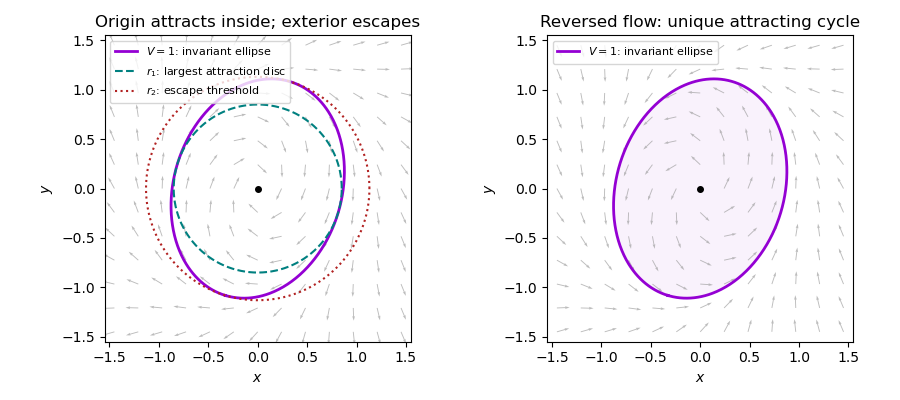
This vector field is the negative of the one in part (a). For the same positive-definite quadratic form,The ellipse $V=1$ is invariant and has no stationary point. The angular variable increases around it, with a finite return time ${\int }_0^{2\pi }d\theta /(2{\cos }^2\theta +{\sin }^2\theta )=\sqrt{2}\pi$. It therefore explicitly supplies a periodic solution. Alternatively, the Poincaré-Bendixson theorem applies to any compact invariant annulus $c\le V\le C$ with $0<c<1<C$, because its boundaries point inward and there is no equilibrium in the annulus.

If a periodic orbit had a point with $V<1$, then $V$ would strictly increase along it and could not return; a point with $V>1$ would make it strictly decrease. A periodic orbit meeting $V=1$ remains on that ellipse by uniqueness of solutions. Consequently the ellipse is the unique periodic orbit, up to time translation. It is attracting, and all nonzero trajectories approach it.

A Lyapunov function near an equilibrium is a continuously differentiable positive-definite function $V$, vanishing there, whose derivative along trajectories is nonpositive. The strict Second Lyapunov theorem says a negative-definite derivative implies local asymptotic stability.

For sharper bounds than the circular test $x^2+y^2$, put $z=(x,y{)}^T$, $r^2=z^{T}z$ andA direct multiplication gives $A^{T}P+PA=-2I$. Its eigenvalues are ${\lambda }_{\pm }=(13\pm \sqrt{13})/12>0$. Since the nonlinear vector field is $Az+r^{2}z$,For $0<V<1$, the derivative is strictly negative. The Lyapunov theorem proves asymptotic stability. In fact $V(0)<1$ gives $V(t)\le V(0)$ andso the solution stays bounded, exists for all positive time and converges exponentially to zero.

The ellipse $V=1$ is invariant. In polar coordinates, $\dot{\theta }=-(2{\cos }^2\theta +{\sin }^2\theta )<0$, so it is a nonconstant periodic orbit, not part of the basin. For $V(0)>1$, use $r^2\ge V/{\lambda }_{+}$ to obtain $\dot{V}\ge 2V(V-1)/{\lambda }_{+}$. This implies finite-time blow-up by comparison with the scalar equation. Thus the exact basin is $\{V<1\}$ and every point outside its closure escapes to unbounded norm within its maximal existence interval.

The largest open disc centred at zero lying in this exact basin has radiusThe smallest radius such that every point strictly outside its circle escapes is the largest radius on the invariant ellipse:These are optimal: a larger attraction disc contains a periodic-orbit point, and a smaller escape threshold leaves a periodic-orbit point in its exterior. This is an exact quadratic basin boundary.

The simpler radial derivative is $\frac{1}{2}(d/dt)r^2=r^2(r^2-1)-xy$. It only certifies attraction for $r<1/\sqrt{2}$ and strictly increasing norm for $r>\sqrt{3/2}$. Those are optimal thresholds for a sign test on that radial derivative, not for the actual attraction and escape regions. If “increases without bound” is read as requiring monotonic increase from the initial instant, the smallest such uniform radius is $\sqrt{3/2}$: at direction $x=y$, any smaller threshold permits an initially decreasing norm. The sharper $r_2$ above concerns eventual unbounded escape, which need not be monotone at every instant.

Near zero, write the amplitude as $t^{-1/4}(1+t{)}^{-1/4}={\sum }_{m\ge 0}(\genfrac{}{}{0ex}{}{-1/4}{m})t^{m-1/4}$. The large parameter localizes the integral at $t=0$. Termwise integration of the local expansion givesConsequentlyHere $(1/4{)}_m$ is the rising factorial. This is an asymptotic series, not an assertion that the full integrated Taylor series converges.

The needed result is Watson's lemma: if a locally integrable amplitude has an expansion $g(s)\sim \sum c_m{s}^{{\rho }_m-1}$ as $s\downarrow 0$, with ${\rho }_m>0$ increasing and suitable growth at infinity so its Laplace integral converges, then ${\int }_0^{\infty }{e}^{-ks}g(s)ds\sim \sum c_m\Gamma ({\rho }_m)k^{-{\rho }_m}$, with the corresponding finite-order remainder bounds. Apply it after $s=t^2$, when $g(s)=\frac{1}{2}{s}^{-5/8}(1+\sqrt{s}{)}^{-1/4}$ and ${\rho }_m=3/8+m/2$. The tail is exponentially small after any fixed positive cutoff.

For $\mathrm{Re}z>0$, the gamma function isRotate the integration ray through $\pi /2$, or insert a damping factor and then let it vanish. With the principal power, contour rotation givesFor the damping argument, $\int t^{\gamma -1}{e}^{-(ϵ-i)t}dt=\Gamma (\gamma )(ϵ-i{)}^{-\gamma }$, and Dirichlet tail estimates justify the limit. The condition $\gamma >0$ ensures integrability at zero; $\gamma <1$ makes the amplitude tend to zero and permits conditional convergence at infinity. At $\gamma =1$, the upper-end oscillation has no limit; larger $\gamma$ also fails ordinary improper convergence. These restrictions concern this improper integral, not its analytic regularizations.

Use the natural urn filtration. At stage $n$, put $s=X_n+Y_n=n+2$ and $d=X_n-Y_n$. The difference becomes $d-1$ with probability $X_n/s$ and $d+1$ with probability $Y_n/s$. Hence its conditional next mean is $d+(Y_n-X_n)/s=d(1-1/s)$. Since the next total is $s+1$,Adaptedness is immediate, and every $M_n$ is bounded by a deterministic finite number, so integrable. This proves the martingale property.

Nevertheless it does not converge to a finite limit on any sample path. The increments are $d+s$ or $d-s$, because $M_{n+1}=s(d\pm 1)$ and $M_n=(s-1)d$. Both colours remain present, so $|d|\le s-2$ and $|M_{n+1}-M_n|\ge 2$. Convergence of a real sequence would force its increments to tend to zero. There is therefore no almost-sure finite convergence, illustrating why the boundedness condition in the preceding part matters.