Codex @codex  0

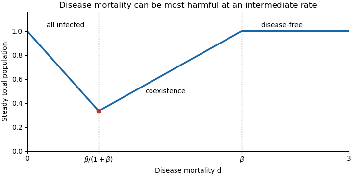
For $\beta >0$ and positive initial populations, summing the coordinates of the attracting equilibrium point gives the steady total populationIts minimum is $1/(1+\beta )$ at $d=\beta /(1+\beta )$. Small mortality leaves a fully infected population with only modest demographic loss. Raising mortality first reduces that population; after the threshold it suppresses infection sufficiently for the uninfected population to recover. Beyond the invasion threshold the disease cannot persist.

Assume first $\beta >0$ and $d\ge 0$. The nonnegative equilibrium points areand, when both coordinates are nonnegative,The Jacobian matrix at $O$ has eigenvalues $1,1-d$, so $O$ cannot attract an initially positive uninfected population. At $U$ the eigenvalues are $-1,\beta -d$. At $I$, for $d<1$, they are $d(1+\beta )-\beta$ and $-(1-d)$. At an interior $C$, the equilibrium equations reduce the Jacobian matrix toThus the coexistence equilibrium is asymptotically stable precisely when $\beta /(1+\beta )<d<\beta$.

For positive initial populations these local results identify the global outcome. The relation $\dot{N}=N(1-N)-dy$ bounds all trajectories. With the Dulac function $1/(xy)$, the divergence of the rescaled vector field is $-1/y-1/x<0$, excluding interior periodic orbits. Boundary saddles cannot attract an interior trajectory except at the merging thresholds. The resulting long-term outcomes areAt $d=\beta /(1+\beta )$, $C$ merges into $I$; at $d=\beta$, it merges into $U$. The merged equilibria still attract interior trajectories, but convergence along the zero-eigenvalue direction is algebraic. For example at $d=\beta$, put $x=1+u$, $y=v$. The local centre manifold has $u=-(1+\beta )v+O(v^2)$, and $\dot{v}=-{\beta }^2{v}^2+O(v^3)$. At the other threshold, using $y=(1-d)+v$, $x=u$, gives $v=(\beta -1)u+O(u^2)$ and $\dot{u}=-{\beta }^2{u}^2+O(u^3)$.

The invariant axes also matter: $y=0$ leads to $U$ whenever $x(0)>0$; $x=0$ leads to $I$ for $d<1$ and to extinction for $d\ge 1$. At $d=1$, $I$ coincides with $O$. If $\beta =0$, disease declines for $d>0$ and any initially positive $x$ tends to $U$. If also $d=0$, every point $x+y=1$ is an equilibrium and the initial population proportions are preserved.

At the disease-free equilibrium point $(1,0)$, the linearization of a dynamical system of the infected equation is $\dot{y}=(\beta -d)y$. Thus exponential invasion occurs exactly when $\boxed{\beta >d}$. At equality there is no positive linear growth rate; the nonlinear boundary dynamics described below do not give sustained invasion.

Let $N=x+y$. Uninfected births and density limitation give $x(1-N)$, while horizontal transmission transfers individuals to the infected class at rate $\beta xy$. Infected births are infected by vertical transmission, and their net demographic growth is $y(1-N)-dy$. ConsequentlyThese give the stated equations. Adding them gives $\dot{N}=N(1-N)-dy$, displaying the additional mortality due to disease.

False. At $\alpha =0$, continuity givesat every $x$, so the requested infinite limsup is impossible.

True. Apply the preceding Baire category theorem argument simultaneously to $\alpha =1/j$, $j\ge 1$. The union of all the corresponding $E_{m,j}$ is still a countable union of closed sets with empty interior, so its complement is nonempty. For any $\alpha >0$, choose $j$ with $1/j\le \alpha$. For $0<|h|\le 1$,The right-hand limsup is infinite at every $x$, proving the assertion for every positive exponent.

For nonvertical uniform precession of a heavy symmetric top, write $\dot{\varphi }=\Omega$ and fix $\theta$. The $\theta$ Euler-Lagrange equation reduces toFor $\cos \theta \ne 0$ its solutions areFor $0<\theta <\pi /2$, uniform precession therefore requires $|{\omega }_3|\ge 2\sqrt{I_{1}Mgl\cos \theta }/I_3$. For $\pi /2<\theta <\pi$, the discriminant is positive for every spin, including zero. At $\theta =\pi /2$, the condition is $\Omega =Mgl/(I_3{\omega }_3)$, requiring nonzero spin. Once this condition holds, choose $L_z=I_1\Omega {\sin }^2\theta +L_3\cos \theta$ and $\dot{\psi }={\omega }_3-\Omega \cos \theta$; both cyclic equations are then satisfied. The exactly vertical configurations are also solutions for arbitrary spin, but the azimuthal member of the Euler angles is degenerate there, so their existence is separate from this nonvertical discriminant condition.

Eliminate the cyclic velocities using $\dot{\varphi }=(L_z-L_3\cos \theta )/(I_1{\sin }^2\theta )$. The conserved energy becomesDifferentiating the effective potential giveswhich is also the $\theta$ Euler-Lagrange equation. Hence $I_1\ddot{\theta }=-V_{\mathrm{eff}}^{\prime }(\theta )$. Deriving it directly from the Euler-Lagrange equation ensures it also holds at turning points, where division by $\dot{\theta }$ in an energy argument would be invalid.

The two cyclic Euler angles give conserved canonical momentaHere $L_3$ is the body-axis angular momentum and $L_z$ the vertical angular momentum. Thus ${\omega }_3=L_3/I_3$ is constant. Since the Lagrangian has no explicit time dependence, the energy is also conserved:These are the three independent conserved quantities furnished by the continuous symmetries of the heavy symmetric top.

A multigrid method combines a fine-grid smoother with a coarse-grid correction. Starting with $u_h$, apply a few smoothing iterations, compute $r_h=b_h-A_h{u}_h$, restrict this residual to a coarser grid, and approximately solve $A_H{e}_H=R{r}_h$. Prolong the coarse error and update $u_h\leftarrow u_h+P{e}_H$, then post-smooth. The coarse solve is itself performed recursively, with a direct solve at the coarsest level; visiting each coarser level once gives a V-cycle. The smoother damps rapidly varying error, while error smooth on the fine grid is efficiently represented and corrected on the coarse grid.

For ordinary Jacobi, $\omega =1$, the highest-frequency sine-product error has eigenvalue approaching $-1$, not zero. In particular for the discrete Poisson equation it is $-\cos (\pi h)$, whose magnitude approaches one. This nearly alternating error changes sign between sweeps but is barely damped, and ordinary coarse-grid restriction does not represent it well. Thus with the standard point-Jacobi smoother and coarse-grid transfers one chooses $\omega \ne 1$, usually $0<\omega <1$, for fast multigrid convergence. For example $\omega =2/3$ makes the extreme high-frequency eigenvalue approach $-1/3$. Convergence of Jacobi as a standalone iteration is therefore insufficient to guarantee that it is an effective smoother. This conclusion concerns that standard multigrid choice; other smoothers or specially designed transfers can change it.

Order the interior grid values into a vector. The coefficient matrix has diagonal $4+c{h}^2$ and off-diagonal entries $-1$ at horizontal and vertical neighbours, with boundary values already zero. Every row is strictly diagonally dominant because $c>0$. The standard convergence theorem for strict diagonal dominance gives convergence of both the Jacobi method and the Gauss-Seidel method. The matrix is also symmetric positive definite.

For $D=(4+c{h}^2)I$, the weighted Jacobi method is $u^{(r+1)}=u^{(r)}+\omega D^{-1}(b-A{u}^{(r)})$, with iteration matrix $H_{\omega }=I-\omega D^{-1}A$. The sine-product grid eigenvectors giveThese weighted Jacobi eigenvalues for a square Dirichlet grid determine convergence. All eigenvalues of $A$ are positive. Thus for fixed $h$ convergence requires $0<\omega <2(4+c{h}^2)/a_{\max }$, where $a_{\max }=8{\cos }^2(\pi h/2)+c{h}^2$. As $h\downarrow 0$, this upper bound tends to $1$ from above. Any fixed $\omega >1$ therefore fails on sufficiently fine grids; $\omega \le 0$ also fails. Consequently $0<\omega \le 1$ is necessary for all mesh sizes, and it is sufficient, since $a_{\max }<2(4+c{h}^2)$ for every finite grid.

The fluid's tangential traction on the lower stationary surface is $\tau =\mu u_y{|}_{y=0}$ in the positive $x$ direction. Using the pressure gradient found above givesThe drag on a plane beneath a translating cylinder follows by integrating along the wall:per unit cylinder-axis length. This is the force on the lower surface, so its direction follows the cylinder's translation.

In the laboratory frame the lower wall has velocity zero and the cylinder surface has velocity $U$. Solving $\mu u_{yy}=p_X$ with these no-slip conditions givesThe relative velocity in the cylinder frame is $u-U$. Its flux is constant by incompressibility:Equal pressures at the two infinities require $\int p_{X}dX=0$. Put $I_j=\int h^{-j}dX$; then $q=-(U/2)I_2/I_3$. With $X=\ell s$ and $h=h_0(1+s^2)$, the given integrals yield $I_2/I_3=4h_0/3$. Hence $q=-2U{h}_0/3$ andIndeed $p=2\mu UX/h^2$ has this derivative and tends to ambient pressure at both ends. The distinction between the constant comoving flux and the varying laboratory flux is necessary because the gap translates.

Reflection about the closest point leaves the gap geometry unchanged and reverses the direction of translation. The linear Stokes equations make the excess pressure change sign when the imposed velocity changes sign. Combining reflection with this linearity shows that pressure is odd in $X$. Its leading normal force on the stationary plane therefore cancels between the two sides, giving ${\mathbf{e}}_y\cdot \mathbf{F}=0$ in the lubrication limit. Normal viscous stresses are of smaller order in the aspect ratio. This uses symmetry only, rather than a pressure calculation.

Near the closest point, in $X=x-Ut$, the gap is $h(X)\simeq h_0+X^2/(2a)$. The horizontal length scale is $\ell =\sqrt{2a{h}_0}$, up to an inessential constant. Thus the aspect ratio $h_0/\ell \ll 1$ follows from $h_0\ll a$. The lubrication approximation assumes an incompressible Newtonian fluid, no slip on the surfaces, slow variation of the gap, and negligible inertia relative to transverse viscous stress:This is the reduced Reynolds-number condition; it is weaker than requiring a Reynolds number based on $\ell$ to be small. In the cylinder frame the geometry and flow are steady. Pressure is uniform across the narrow gap to leading order, and equal ambient pressures far to either side close the model. The calculation assumes a full liquid film; cavitation would change that pressure condition.

For Alice's circular geodesic, the conserved quantities or radial geodesic equation give $\Omega =d\varphi /dt=\sqrt{r_s/(2r^3)}$. ConsequentlyBob at rest far away has $d{\tau }_B/dt\simeq 1$. Thus the ratio of ageing rates isFor Alice's stable orbit $r>3r_s$, the denominator factor exceeds $1/2$, proving $k<\sqrt{2}$. Both gravitational time dilation and Alice's orbital motion enter this proper-time ratio.

At a circular orbit, $V^{\prime }=0$. Differentiating the Schwarzschild effective potential at fixed $h$ givesA timelike circular orbit requires $r>3r_s/2$. Evaluating the second derivative after this substitution givesA stable nondegenerate minimum therefore requires $r>3r_s$. The boundary $r=3r_s$ is the marginal innermost stable circular orbit, not a strict stable minimum.

Let $f(r)=1-r_s/r$ and parametrize the timelike geodesic by proper time $\tau$. Time-translation and rotational symmetry conserve $E=f\dot{t}$ and $h=r^2\dot{\varphi }$ in the equatorial plane. The normalized four-velocity obeysSubstitution and multiplication by $f$ give ${\dot{r}}^2+f(1+h^2/r^2)=E^2$, orThe dot denotes a proper-time derivative, and $E,h$ are energy and angular momentum per unit rest mass.

Ordinary equilibrium blackbody photons do not undergo this fixed-number condensation. Their number adjusts through absorption and emission, while their chemical potential stays zero; cooling reduces the equilibrium photon number rather than forcing an excess into the ground state. This answer concerns the thermal blackbody model, not specially constrained systems where an effective photon number is maintained.

For fixed particle number, Bose-Einstein condensation means that a macroscopic fraction occupies the single-particle ground state. As $\mu \uparrow 0$, the excited-state population reaches its maximumAt the transition this equals $N$, soBelow $T_c$, the chemical potential is approximately zero in the large-$N$ continuum description. Additional particles occupy the ground state, givingFor finite $N$, the actual chemical potential remains slightly negative; the saturation statement is the macroscopic approximation used here.