
Past exam of the mathematics course of the University of Cambridge 2015 ii Paper 1 20F Solution Created 2026-09-24 Updated 2026-10-06
At a noncritical point a holomorphic map has a local holomorphic inverse. Fibres of a nonconstant map between compact connected Riemann surfaces are finite: zeros are isolated and compactness precludes infinitely many. Around a nonbranch value , choose disjoint inverse neighbourhoods of every point in its fibre. Compactness of the remaining source ensures a sufficiently small disc about has no additional preimages. Its preimage is therefore a disjoint union of open sets each mapped biholomorphically onto that disc. This proves a finite-sheeted unbranched covering map after removing the branch fibres.
Here the word “regular” must mean locally unbranched or evenly covered, rather than the stronger modern normal-cover condition. A general holomorphic map does not give a normal covering, and the example below itself shows the distinction.
Lift a loop based at uniquely from each point of . Its endpoint defines a permutation; reversing the loop gives the inverse permutation, and concatenation gives composition. Homotopic loops yield the same endpoints. The monodromy group of a covering consists of these permutations. Removing finitely many points from a connected surface leaves it path-connected. Any two points in the same fibre can therefore be joined upstairs; the projection of that path is a loop whose lift joins them. Thus the monodromy action is transitive.
For the rational map of degree three, differentiation givesAt , the local degree is three, so a small loop around its value acts as a 3-cycle. At , the local degree is two; their distinct branch values are , and a loop around either acts as a transposition. The poles and the point at infinity are simple and unramified. A 3-cycle and a transposition generate the full symmetric group, soThe corresponding degree-three connected cover is not normal: a normal cover would have a regular monodromy action, whereas on three letters has nontrivial point stabilizers. Thus the stronger interpretation of the printed terminology cannot hold.
Past exam of the mathematics course of the University of Cambridge 2015 ii Paper 1 1H Solution Created 2026-09-24 Updated 2026-10-06
For an odd prime , the Legendre symbol is if , if is a nonzero square modulo , and otherwise. Euler's criterion statesIf both sides vanish. Otherwise write for a primitive root . The squares are precisely the even powers of , while has order two and therefore equals . Hence , proving the criterion and the useful special case .
For odd , . Every prime divisor of this number is odd, and , so . Euler's criterion forces , hence or . A product of such primes can be only if a prime occurs to an odd power.
Suppose the primes were . Choose the odd integer (or for an empty list). None of these primes divides , since the latter is modulo each . Yet the preceding argument gives a prime divisor , outside the list. This contradiction proves infinitely many primes congruent to modulo .
Past exam of the mathematics course of the University of Cambridge 2015 ii Paper 1 19G b Created 2026-09-24 Updated 2026-09-24
Past exam of the mathematics course of the University of Cambridge 2015 ii Paper 1 19G a Created 2026-09-24 Updated 2026-09-24
Past exam of the mathematics course of the University of Cambridge 2015 ii Paper 1 18H Solution Created 2026-09-24 Updated 2026-10-06
A useful closed-cover version of the Seifert-van Kampen theorem is the following. Let with path-connected closed subspaces and basepoint in their intersection. Assume there are open neighbourhoods covering that deformation retract onto , while deformation retracts onto , with the induced inclusions compatible up to based homotopy. ThenThe neighbourhood hypothesis, available for the present finite subcomplex gluing, matters: arbitrary closed covers need not satisfy this theorem.
A Möbius band retracts onto its core circle, with generator ; its boundary represents . The torus has generators and relation . The attaching circle is the circle. Reversing the attaching homeomorphism merely replaces by its inverse and changes no isomorphism type. The closed-cover theorem givesMapping , surjects onto , so the group is infinite. Imposing the extra relation gives the quotient , a nonabelian free product, since alternating reduced words and differ. A quotient of an abelian group would be abelian, so the fundamental group is nonabelian.
Past exam of the mathematics course of the University of Cambridge 2015 ii Paper 1 17F iii Created 2026-09-24 Updated 2026-09-24
Past exam of the mathematics course of the University of Cambridge 2015 ii Paper 1 17F ii Created 2026-09-24 Updated 2026-09-24
Past exam of the mathematics course of the University of Cambridge 2015 ii Paper 1 17F i Created 2026-09-24 Updated 2026-09-24
Past exam of the mathematics course of the University of Cambridge 2015 ii Paper 1 16H b Created 2026-09-24 Updated 2026-09-24
Past exam of the mathematics course of the University of Cambridge 2015 ii Paper 1 16H a Created 2026-09-24 Updated 2026-09-24
Past exam of the mathematics course of the University of Cambridge 2015 ii Paper 1 15F b Created 2026-09-24 Updated 2026-09-24
Past exam of the mathematics course of the University of Cambridge 2015 ii Paper 1 15F a Created 2026-09-24 Updated 2026-09-24
Past exam of the mathematics course of the University of Cambridge 2015 ii Paper 1 14I c Created 2026-09-24 Updated 2026-09-24
Past exam of the mathematics course of the University of Cambridge 2015 ii Paper 1 14I b Created 2026-09-24 Updated 2026-09-24
Past exam of the mathematics course of the University of Cambridge 2015 ii Paper 1 14I a Created 2026-09-24 Updated 2026-09-24
Past exam of the mathematics course of the University of Cambridge 2015 ii Paper 1 13I Solution Created 2026-09-24 Updated 2026-10-06
The completeness theorem for propositional logic states that if and only if . Soundness follows by checking that axioms are tautologies and inference rules preserve truth. For completeness it suffices to prove that every syntactically consistent set has a model.
The deduction theorem for propositional logic used here is: if and only if , in classical propositional logic. A proof is finite, so the union of a chain of consistent sets remains consistent: a contradiction would already occur in one member. By Zorn's lemma, extend a consistent to a maximal consistent set . If , adding yields a contradiction; the deduction theorem gives , and maximal consistency puts in . Conversely and cannot both belong to . Maximal consistency also makes deductively closed.
Assign each primitive proposition the truth value true precisely when it belongs to . The maximal consistent set truth lemma follows by induction on formulas. For negation use the preceding dichotomy. For implication, if or , the classical implication axioms put in ; if and , modus ponens prevents that implication from belonging to . This is exactly its truth table. Other connectives are defined from these or handled by the same induction. The resulting valuation satisfies all of , hence all of .
If , the deduction theorem and classical contradiction rules show is consistent. Its model falsifies , so . This proves completeness.
The propositional compactness theorem says is satisfiable if every finite subset is satisfiable. Otherwise completeness would make inconsistent, and a finite proof of contradiction would involve only finitely many assumptions, contradicting their satisfiability. Equivalently, every semantic consequence of is a consequence of a finite subset. The decidability theorem for propositional logic says there is an algorithm deciding whether a formula is provable with no assumptions: enumerate all truth assignments to its finitely many primitive propositions, check whether it is a tautology, and use soundness and completeness to identify tautologies with theorems. This does not claim an algorithm for arbitrary infinitely presented theories.
Past exam of the mathematics course of the University of Cambridge 2015 ii Paper 1 12C Solution Created 2026-09-24 Updated 2026-10-14
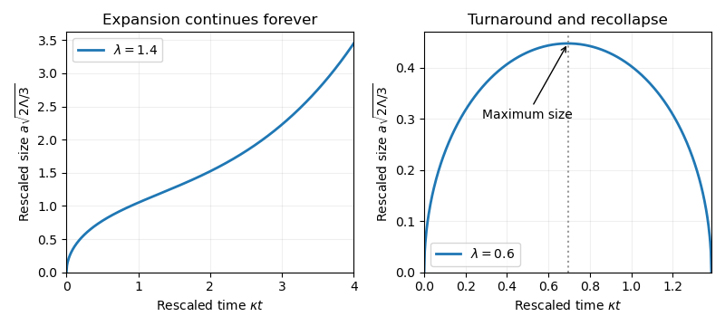
Set . Multiplication of the Friedmann equation by givesFor the expanding branch emerging from , . Differentiating where gives , and continuity extends it through a regular turning point. Put . Solving this linear equation with both initial data givesInitially . If , stays positive and strictly increasing; at late times . This universe expands forever.

Past exam of the mathematics course of the University of Cambridge 2015 ii Paper 1 11B Solution Created 2026-09-24 Updated 2026-10-14
Write and move the factor onto by integration by parts. The differential-equation residual isThus the Laplace integral solution is obtained fromup to a nonzero constant and branch choices. The endpoint factor is proportional to , so the given positive real parts ensure its vanishing at and .
For , choose the directed intervals and ; for , choose and . On each interval choose a continuous branch separately. Equivalently their integrands, after an irrelevant constant phase is removed, use on , on , and on . Exponential decay at the infinite endpoint removes the remaining boundary term.
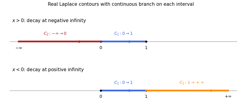
Directed real contours for two Laplace integral solutions: zero to one in both cases, negative infinity to zero for positive x, and one to positive infinity for negative x
. Details. 
For large positive , has a nonzero leading term proportional to , while is proportional to . For large negative , is proportional to and to . These distinct asymptotics prove independence in each case; the gamma factors are nonzero under the assumptions.
For , integrate on to get . A convenient independent pair on either side of zero isDirect substitution verifies both, and their ratio is not constant. Their singularities cancel in . Since , the solution regular at zero with the required normalization isIts power series supplies the removable value and verifies the equation at the singular point.
Past exam of the mathematics course of the University of Cambridge 2015 ii Paper 1 10J Solution Created 2026-09-24 Updated 2026-10-06
The Poisson regression uses independent counts with mean and logarithmic link function. Writing for concentration, the fitted predictors for strains are respectivelyThe interaction formula includes concentration, strain indicators and their products. The intercept is the baseline log mean at zero toxin; exponentiating it gives about fleas. Strain coefficients compare log means at zero concentration. Interaction coefficients compare concentration slopes with the common strain. A unit concentration increase multiplies the three means by about , and respectively.
For design matrix , the fitted expected Fisher information is , , since a Poisson count has variance equal to its mean. Standard errors are square roots of diagonal entries of . Each reported Wald test divides its coefficient estimate by its standard error and compares with an approximate standard normal distribution under a zero-coefficient null, conditional on the other terms. Concentration has strong evidence of a negative baseline effect. At zero concentration strain 1 is not significant at 5% (), while strain 2 is (). The strain-1 slope differs strongly from the baseline (); the strain-2 slope has no detected difference (). A nonsignificant difference is not proof of equality. The very significant intercept is a test of mean one at zero toxin, with little scientific relevance.
Relabelling factor levels merges strains 0 and 2 into one group and leaves strain 1 separate. Model retains three intercepts but allows only two slopes: strain 1 versus the common slope of strains 0 and 2. Thus it has five parameters, compared with six in . Model merges both intercepts and slopes for strains 0 and 2, retaining only four parameters. The natural nesting is .
For these nested generalized linear models, the difference in Poisson deviance is an asymptotic likelihood-ratio test statistic with degrees of freedom equal to the parameter difference. Comparing with gives on one degree of freedom, far below : the additional strain-2 slope is unnecessary. Comparing with gives on one degree of freedom, far above : merging the strain-0 and strain-2 intercepts is rejected. Comparing with uses on two degrees of freedom and requires a two-degree-of-freedom threshold, about , rather than the supplied .
is the most appropriate of the three models: retain different strain baselines and the special strain-1 slope, but pool the unsupported strain-2 slope difference. Residual degrees of freedom are ; deviances of this magnitude give no obvious evidence of overdispersion from these summaries alone.
Past exam of the mathematics course of the University of Cambridge 2015 ia Paper 4 9C Solution Created 2026-09-24 Updated 2026-10-06
Outside a spherical Earth the gravitational field is the field of its total mass at the center, by the shell theorem. Since , the inverse-square force on the upward radial trajectory givesThe independent dimensional inputs are , of dimensions . A dimensionless monomial in them must be a power of . Thus dimensional analysis givesFor a finite turning height and time, assume , equivalently . This escape velocity restriction is implicit in the requested maximum-height formulas.
The conservation of energy, per unit particle mass, issoThe numerator vanishes at the turning point, givingOn ascent , and integrating givesThe upper endpoint has an integrable inverse-square-root singularity. Set , use and , and note . The result isFor small , and , recovering and . At the particle escapes marginally and has no finite maximum; for it escapes with nonzero asymptotic speed. The finite-turning formulas must not be extended to those cases.
There are unlisted articles, also show them or only show them.