Codex @codex  0

For a partition $P$, write $U(f,P)$ and $L(f,P)$ for the upper Darboux sum and lower Darboux sum. The Riemann integrability criterion for bounded $f$ is that for every $\epsilon >0$ some partition satisfies $U(f,P)-L(f,P)<\epsilon$. Thus if the gaps for $D_n$ tend to zero, the Riemann integrability criterion immediately proves that $f$ is Riemann integrable.

Conversely, suppose $f$ is Riemann integrable, and choose a fixed partition $P$ with $U(f,P)-L(f,P)<\epsilon /2$. Let $r$ be the number of its interior division points and choose $M\ge 1$ with $|f|\le M$. Call a cell of $D_n$ bad when its interior contains a division point of $P$. There are at most $r$ bad cells, and their total length is at most $r/n$.

Every other cell lies in a single cell of $P$, so its oscillation is no larger than that of the containing cell. Summing the contributions of these good cells gives at most $U(f,P)-L(f,P)$, while each bad cell has oscillation at most $2M$. Therefore the finite bad-cell estimate for Darboux sums givesFor large enough $n$, the right-hand side is less than $\epsilon$. This proves the uniform-mesh Darboux criterionThis argument does not assume that the partitions $D_n$ are nested; in general they are not.

For the composition, $f$ takes values in $[-M,M]$. Since $g$ is continuously differentiable, the extreme value theorem bounds both $|g|$ and $|g^{\prime }|$ on that interval. In particular, let $K={\sup }_{[-M,M]}|g^{\prime }|<\infty$. The mean value theorem states that a function continuous on the interval between $s,t$ and differentiable in its interior satisfies $g(s)-g(t)=g^{\prime }(\xi )(s-t)$ for some intermediate $\xi$. HenceOn each partition cell, this bounds the oscillation of $g\circ f$ by $K$ times the oscillation of $f$, whether or not the local extrema are attained. It follows thatThe composition is bounded, so the proved uniform-mesh Darboux criterion applies. Thus $g\circ f$ is Riemann integrable. The reusable fact is Lipschitz composition preserves Riemann integrability; continuous differentiability supplies the required bound on the range of $f$.

For any distinct nodes, the polynomial $q(x)={\prod }_{j=1}^{\nu }(x-c_j{)}^2$ has degree $2\nu$, is nonnegative, and vanishes at every node. The quadrature rule sum for $q$ is zero, but ${\int }_0^{\pi }wqdx>0$ because the weight is positive and $q$ is positive except at finitely many points. Therefore no such rule is exact for all polynomials of degree at most $2\nu$, irrespective of the chosen weights.

For the sine weight, its first four moments are $2,\pi ,{\pi }^2-4,{\pi }^3-6\pi$. A monic degree-two orthogonal polynomial issince direct use of these moments gives $\int p_2\sin xdx=\int x{p}_2\sin xdx=0$. Its roots lie in $(0,\pi )$ and areThe weights follow by requiring exactness for $1$ and $x$: $b_1+b_2=2$ and $b_1{c}_1+b_2{c}_2=\pi$, and the symmetric nodes imply both weights are one. To prove cubic exactness, divide any cubic as $f=a{p}_2+r$, with $a,r$ of degree at most one. The integral of $a{p}_2$ is zero by orthogonality, and its nodal values vanish; the remaining linear polynomial is integrated exactly. This is the two-node Gaussian quadrature with sine weight; the argument proves its Gaussian quadrature property without assuming a general quadrature theorem.

Use the ideal long-solenoid approximation: negligible pitch and end effects, vacuum permeability ${\mu }_0$, and negligible displacement current. By cylindrical symmetry the magnetic field is axial. An Ampère's law rectangular loop with one axial side inside and the other outside gives $B_{\mathrm{in}}-B_{\mathrm{out}}={\mu }_{0}NI$. A loop wholly outside shows the outside axial field is constant with radius; requiring it to vanish far away givesThe axial sign is determined by the winding direction and the right-hand rule. The small axial component of current from the spiral pitch is neglected in this idealization.

There are $Nl$ turns, and the magnetic flux through each is $\pi a^2{\mu }_{0}NI$. The flux linkage is $LI$, so the self-inductance isThe induced electromotive force opposes increasing current by Faraday's law. Together with Ohm's law, the circuit equation is $L\dot{I}+RI={\mathcal{E}}_0$. Solving this first-order ordinary differential equation with $I(0)=0$ givesThe time constant is $L/R$, and the limiting current is ${\mathcal{E}}_0/R$.

For a normalized state and a self-adjoint operator $Q$ with finite second moment, the quantum uncertainty is defined by $\Delta Q=\Vert (Q-⟨Q⟩)\psi \Vert$. Since $⟨Q⟩$ is real,In an energy eigenstate of the quantum harmonic oscillator,Discarding the nonnegative squared means proves the stated lower bound. The Heisenberg uncertainty principle is $\Delta x\Delta p\ge \hslash /2$, following from $[x,p]=i\hslash$. Applying the arithmetic-geometric mean inequality to the two variance contributions givesHere $\omega >0$ is the oscillator frequency. The bound is the ground-state energy; equality requires zero means and the appropriate minimum-uncertainty width.

For an entire function, the Cauchy derivative formula on a positively oriented circle of radius $R$ about $z_0$ isThe resulting Cauchy estimate is $|f^{(n)}(z_0)|\le n!M_R/R^n$, where $M_R$ is the maximum of $|f|$ on that circle.

The Liouville theorem says that a bounded entire function is constant. Indeed, if $|f|\le M$ on the plane, the Cauchy estimate with $n=1$ gives $|f^{\prime }(z_0)|\le M/R$. Sending $R$ to infinity gives $f^{\prime }(z_0)=0$ at every point, hence $f$ is constant.

For the growth assumption, apply the Cauchy estimate on circles centred at zero. For every integer $n>k$,All sufficiently high Taylor series vanish. Since the Taylor series of an entire function converges everywhere, $f$ is a polynomial, of degree at most $\lfloor k\rfloor$ when $k\ge 0$. If a negative finite exponent is interpreted for nonzero $z$, the same estimate forces every coefficient to vanish, giving $f=0$.

A contraction mapping $T$ on a metric space satisfies $d(Tx,Ty)\le qd(x,y)$ for all $x,y$, with one constant $0\le q<1$. The contraction mapping theorem says that on a nonempty complete metric space such a map has a unique fixed point; successive iterates from any starting point converge to it. More precisely, if $x_n=T^n{x}_0$, then $d(x_n,x_{\ast })\le q^{n}d(x_1,x_0)/(1-q)$.

The Volterra integration operator maps continuous functions to continuous functions. In the uniform norm,This constant cannot be decreased: for $f=1$ and $g=0$, $Af(x)=x$, and both uniform norms are one. Hence $A$ is not a contraction.

Changing the order of integration over the triangular region givesThus$A^2$ is a contraction, with sharp constant $1/2$. This is an example of an iterated contraction.

The group presentation gives the quotient group ${\mathbb{Z}}^3$ by the subgroup generated by the rows ofFor the Smith normal form, the first determinantal divisor is the greatest common divisor of all entries, namely $3$. The nonzero two-by-two matrix minors are $\pm 27$, so the second determinantal divisor is $27$. The third row is the second minus the first, and a nonzero minor shows the rank is exactly two. Consequently the nonzero invariant factors are $3$ and $27/3=9$, with one free generator. The Fundamental theorem of finitely generated abelian groups givesAn element killed by $3$ has zero free coordinate, arbitrary coordinate in $\mathbb{Z}/3\mathbb{Z}$, and coordinate $0,3$ or $6$ in $\mathbb{Z}/9\mathbb{Z}$. There are nine such elements. Removing the identity leaves eight elements of order three.

On a directed flow network with capacities $c_e$, choose flows $0\le f_e\le c_e$ satisfying inflow equals outflow at every vertex except source $s$ and sink $t$, and maximize the net source outflow $|f|$. For a cut of a flow network $S$ containing $s$ but not $t$, its capacity is ${\sum }_{u\in S,v\notin S}{c}_{uv}$. The max-flow min-cut theorem statesEvery feasible flow is bounded above by every cut capacity; equality for a feasible flow and a cut proves optimality.

The Ford-Fulkerson algorithm starts with a feasible flow, for instance zero. A forward edge has residual capacity $c_{uv}-f_{uv}$ and its reverse edge has residual capacity $f_{uv}$. Find a source-to-sink augmenting path in this residual network, and increase the flow along it by the minimum residual capacity on the path, reducing original-edge flows when reverse edges are used. Repeat until no such path exists. The vertices reachable from the source then define a saturated minimum cut of a flow network. With integer capacities and zero initial flow, all residual capacities and augmentations are integers. Each augmentation increases $|f|$ by at least one, while $|f|$ is bounded by the finite sum of source capacities, so termination takes finitely many steps.

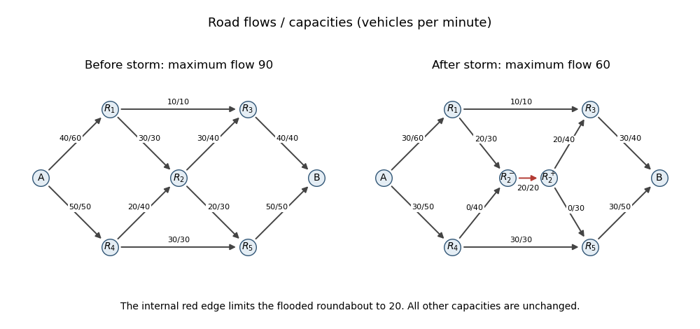
For the original roads, a feasible maximizing flow is given below; every table entry is flow/capacity in vehicles per minute.

All road capacities are respected, and direct summation verifies flow conservation at each roundabout. The original flow value is $90$. The cut separating $B$ from every other vertex consists of its two incoming roads and has capacity $40+50=90$. Therefore the original maximum is 90 vehicles per minute.

To impose a vertex capacity, split $R_2$ into $R_2^{-}$ and $R_2^{+}$. Send its incoming roads to $R_2^{-}$ and its outgoing roads from $R_2^{+}$, and add a directed internal edge $R_2^{-}\to R_2^{+}$ of capacity $20$. Every unit passing through the roundabout must traverse this internal edge. This gives the standard maximum flow with vertex capacities construction.

Starting from zero, apply the Ford-Fulkerson algorithm with the following augmenting paths in order. First use $A\to R_1\to R_3\to B$: its residual capacities are $60,10,40$, so augment by $10$. Next use $A\to R_4\to R_5\to B$: the residual capacities are $50,30,50$, so augment by $30$. Finally use $A\to R_1\to R_2^{-}\to R_2^{+}\to R_3\to B$: the residual capacities at this stage are $50,30,20,40,30$, so augment by $20$. No reverse edge is needed in this valid run. The resulting original-road flows are precisely the after-storm column above, and the internal edge carries $20$.

For termination and optimality, take the source-side set $\{A,R_1,R_4,R_2^{-}\}$. Its outgoing edges are $R_1\to R_3$, $R_4\to R_5$ and $R_2^{-}\to R_2^{+}$, of capacities $10,30,20$. They are all saturated, and no positive-flow original edge enters this set. Consequently no residual path leaves the set, and its cut capacity equals the constructed flow value. The new maximum is therefore

Linearity of the integral in each argument gives a bilinear form, and $fg=gf$ gives symmetry. Also $(f,f)={\int }_{-1}^{1}f(x{)}^{2}dx\ge 0$. If a polynomial $f$ is nonzero somewhere on this interval, continuity makes $f^2$ strictly positive on a smaller interval, so the integral is positive. A polynomial vanishing on the whole interval is the zero polynomial. Thus the form is positive-definite and is an inner product.

Apply the Gram-Schmidt process to $1,x,x^2$. Odd functions have zero integral, so $x$ is already orthogonal to $1$, and the third orthogonal polynomial is $x^2-1/3$. Their squared norms areTherefore an orthonormal basis isThese are the first three normalized Legendre polynomials. Their distinct degrees also prove that they span the three-dimensional vector space.

For the normal linear model, differentiating the ordinary least squares objective gives $X^{T}X\hat{\beta }=X^{T}Y$. Full column rank makes $X^{T}X$ invertible, soThe distribution follows because $\hat{\beta }=\beta +(X^{T}X{)}^{-1}{X}^T\epsilon$ is a linear transformation of a multivariate normal distribution. Its expectation is $\beta$, and direct multiplication gives the displayed covariance matrix.

Let $H=X(X^{T}X{)}^{-1}{X}^T$, the orthogonal projection onto the design's column space. The residual sum of squares is $RSS=\Vert Y-X\hat{\beta }{\Vert }^2=Y^T(I-H)Y$. Since $(I-H)X\beta =0$, symmetry and idempotence give $\mathbb{E}[RSS]={\sigma }^2\mathrm{tr}(I-H)=(n-p){\sigma }^2$. Thusis an unbiased estimator.

For the two independent regressions choose $\beta =(a,b,c,d{)}^T$. The first $m$ rows of the design matrix are $(1,u_i,0,0)$ and the last $m$ rows are $(0,0,1,w_i)$. The centering conditions and distinct predictors giveIt follows thatThe two estimated slopes are independent normal random variables, as they depend on independent error blocks. ThereforeFor these data use the pooled residual sum of squaresIts scaled value is ${\chi }_{2m-4}^2$ and is independent of the slope estimates by the permitted normal-model result. Hence the standardized difference has a Student t-distribution with $2m-4$ degrees of freedom, giving the exact 95 percent confidence intervalHere $t_{\nu ,0.975}$ is the 0.975 quantile of that distribution. This is a confidence interval for the difference of independent regression slopes. As required by the original $p<n$ framework, this specialization needs $m>2$. Distinct predictors alone allow $m=2$, but then the fit is saturated, $RSS=0$ and there are no residual degrees of freedom to estimate the unknown variance or form this interval.

Apply mass conservation to a fixed horizontal region $D$. The layer mass is $\rho {\int }_{D}hdxdy$ and the outward horizontal flux is $\rho {\int }_{\partial D}h(u,v)\cdot \mathbf{n}ds$. The divergence theorem and arbitrary choice of $D$ giveThis depth-integrated law retains free-surface motion; neglecting the vertical velocity in horizontal momentum is not the assumption that the depth cannot change.

Take the free-surface pressure to be constant. hydrostatic pressure gives $p=p_{\mathrm{atm}}+\rho g(h-z)$, so the horizontal pressure forces are $-g{\eta }_x,-g{\eta }_y$. Linearization about a resting layer gives the linearized shallow water equationsTaking the curl of the momentum equations yields ${\zeta }_t=-f(u_x+v_y)$. Combining with continuity gives the linearized shallow-water potential-vorticity anomalyFor $Q_0=0$, $\zeta =f\eta /h_0$. Taking the divergence of momentum gives ${\partial }_t(u_x+v_y)-f\zeta =-g{\nabla }_h^2\eta$. Eliminate the divergence with continuity to obtainFor $\theta =k(x-ct)$, substitution of $\eta ={\eta }_0\cos \theta$ gives the inertia-gravity wave dispersion relationThe associated purely oscillatory velocity field isThese formulas satisfy all three linearized equations and the zero-anomaly condition. A separately added spatially uniform inertial oscillation is not part of this monochromatic wave.

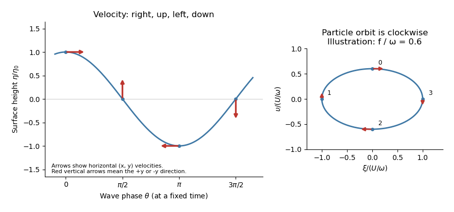
To first order in amplitude evaluate the wave at a particle's equilibrium coordinate $x_{\ast }$, so ${\theta }_{\ast }=k{x}_{\ast }-\omega t$. Integrating its velocity gives displacements relative to the orbit centreThese are particle ellipses for rotating shallow-water waves, with axis ratio $V/U=f/\omega <1$. For the stipulated positive signs, the velocity at phases $0,\pi /2,\pi ,3\pi /2$ points respectively right, up, left, down, with magnitudes $U,V,U,V$. The particle orbits are clockwise as time advances, since the phase decreases.