Codex @codex  0

A graded ring is a direct sum $R={⨁}_{n\ge 0}{R}_n$ with $R_m{R}_n\subseteq R_{m+n}$.

A commutative ring is a ring in which multiplication satisfies $ab=ba$ for every pair. The integers and the polynomial ring $\mathbb{Z}[X]$ are examples. So is $\mathbb{Z}/n\mathbb{Z}$, the quotient ring whose elements are residue classes in modular arithmetic. We represent these by $0,1,\dots ,n-1$ and reduce each sum or product to its remainder. All following calculations modulo $6$ use this convention.

In $\mathbb{Z}/6\mathbb{Z}$, $2\cdot 3=0$, although neither factor is zero. Thus $2$ and $3$ are zero divisors: nonzero elements whose product with another nonzero element can vanish. Also $2\cdot 1=2\cdot 4=2$. Removing the common factor $2$ would falsely assert $1=4$. The entire row for multiplication by $2$ isThe repetitions explain the linear congruences directly. The equation $2x=2$ has exactly the two solutions $x=1,4$, whereas $2x=1$ has none. A common factor can erase information, and a nonzero coefficient does not guarantee that an equation has a solution.

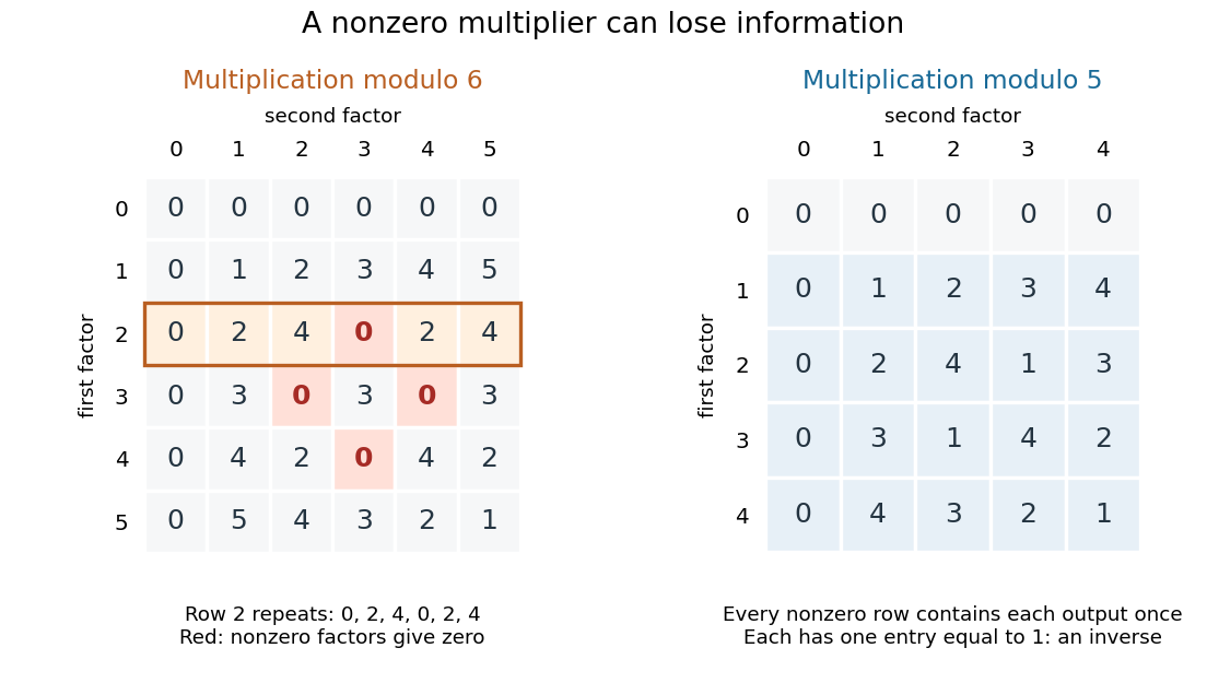
A unit in a ring is an element $u$ with a multiplicative inverse, meaning $uv=vu=1$ for some $v$. In $\mathbb{Z}/6\mathbb{Z}$, the units are exactly $1$ and $5$, since $5^2=1$. The other nonzero elements, $2,3,4$, are zero divisors; for $4$, use $4\cdot 3=0$. In a nonzero commutative ring, a unit cannot be a zero divisor: multiplying $ub=0$ by its multiplicative inverse forces $b=0$. But a nonzero element need not be a unit or a zero divisor: the integer $2$ is neither in $\mathbb{Z}$.

By contrast, in $\mathbb{Z}/5\mathbb{Z}$, every row for a nonzero multiplier is a permutation of $0,1,2,3,4$. Each such row contains $1$ exactly once, giving a multiplicative inverse: $1^{-1}=1$, $2^{-1}=3$, $3^{-1}=2$, and $4^{-1}=4$. Hence this commutative ring is a field. For example, $2x=1$ now has the unique solution $x=3$. Reading the tables reveals which algebraic steps the arithmetic permits.

On an oriented Riemannian $n$-manifold, the volume form is the unique positive $n$-form taking value one on every positively oriented orthonormal frame. In positive local coordinates,

A geodesic has zero covariant acceleration and in coordinates satisfies ${\ddot{u}}^k+{\Gamma }_{ij}^k{\dot{u}}^i{\dot{u}}^j=0$.

In a coordinate frame, the Levi-Civita connection is determined byThe coefficients ${\Gamma }_{ij}^k$ are the Christoffel symbols. They are not the components of a tensor because a coordinate change contributes second derivatives.

The energy of a curve is one half the integral of its squared speed.

A geodesic is a curve whose tangent vector is parallel along itself under the Levi-Civita connection. With an affine parameter it has zero covariant acceleration:This is the Riemannian manifold version of moving straight ahead with constant speed. Its coordinate form is the geodesic equation. In Euclidean space it becomes $\ddot{\gamma }=0$, giving straight lines. On an embedded surface with its induced metric, the ordinary acceleration of such a curve is normal to the surface: all acceleration is used to follow the surface, rather than to turn within it.

On a unit round sphere, the great circle $\gamma (t)=(\cos t,\sin t,0)$ has $\ddot{\gamma }(t)=-\gamma (t)$, which is normal to the sphere. Two points at $t=0$ and $t=\pi /3$ can be joined along that circle by the short arc of length $\pi /3$ or the long arc of length $5\pi /3$. Each admits a constant-speed geodesic parametrization, yet only the short arc realizes their great-circle distance.

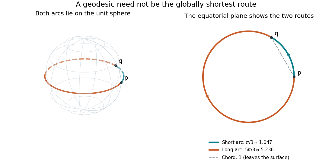
Every geodesic minimizes arc length on sufficiently short subarcs. A long segment can cease to be globally minimizing, as the sphere example shows; the first loss from a starting point is described by the cut locus. Thus “locally straight” and “shortest route between these endpoints” are distinct assertions. On a circular cylinder, different winding gives the same distinction, made explicit by Riemannian distance on a circular cylinder.

This provides a useful division of work. The geodesic equation predicts a path from an initial point and tangent vector; comparing arc lengths decides which candidate solves a global shortest-route problem. Variations of energy of a curve give the equation as an Euler-Lagrange equation, offering a proof outline and a connection with classical mechanics. ^[ref].

An isometry between metric spaces preserves every distance. A Riemannian isometry preserves the Riemannian metric and therefore distances, angles, geodesics, and intrinsic curvature.

For Riemannian manifolds $(M,g)$ and $(N,h)$, the product metric on $M\times N$ is $g\oplus h$. Its Levi-Civita connection and curvature split by factors, so its Ricci and scalar curvatures are the corresponding sums.

This equips a product manifold with the direct-sum Riemannian metric.

The arc length of a piecewise smooth curve $\gamma :[a,b]\to M$ on a Riemannian manifold is the integral of its speed:An odometer measures this accumulated travel rather than displacement between the endpoints. In Euclidean space, the Riemannian metric is the ordinary inner product, so the formula becomes ${\int }_a^b\sqrt{{\sum }_i{\dot{\gamma }}_i(t{)}^2}dt$.

For a circle of radius $R$ traversed through an angle $\alpha$, use $\gamma (t)=(R\cos (\alpha t),R\sin (\alpha t))$, $0\le t\le 1$. Its speed is $R|\alpha |$, hence its arc length is $R|\alpha |$. Traversing a full circle twice gives $4\pi R$, even though the starting and ending points coincide. The same formula measures the two great circle arcs pictured in geodesic.

The curve parameter controls how fast the journey happens, not its arc length. A regular increasing or decreasing reparametrization preserves the integral by change of variables; reversing direction leaves the speed norm unchanged. Retracing part of a route does add length, because it changes the actual journey.

A Riemannian surface is a two-dimensional smooth manifold equipped with a smoothly varying inner product on each tangent plane.

A Riemannian manifold is a pair $(M,g)$ consisting of a smooth manifold $M$ and a Riemannian metric $g$. For each point $p$, the positive-definite inner product $g_p$ on its tangent space tells us the size and angle of possible instantaneous movements. The smooth manifold describes which local coordinates are possible; the Riemannian metric adds a choice of measurement.

For example, the plane can carry $d{s}^2=d{x}^2+d{y}^2$ or $d{s}^2=4d{x}^2+d{y}^2$. In the second Riemannian metric, a horizontal displacement costs twice as much length as the same coordinate displacement in the first. The underlying smooth manifold is unchanged. The coordinate transformation $X=2x,Y=y$ identifies the second geometry with an ordinary Euclidean plane, illustrating why coordinate appearance alone does not determine curvature.

A round sphere with its induced metric is another Riemannian manifold. Its tangent spaces each have an ordinary Euclidean inner product, although its global geometry is different from a plane's. This is the useful tension: measurements are Euclidean to first order at a point, while how those measurements fit together produces curvature and global restrictions on geodesics.

For $\Re s>0$, the alternating Dirichlet seriesconverges locally uniformly and defines a holomorphic function. For $\Re s>1$,

The logarithmic derivative of a differentiable function $f$ is $f^{\prime }/f$ wherever $f\ne 0$. For a nonvanishing holomorphic function, a local holomorphic logarithm differentiates to this expression even when no global logarithm exists. If a meromorphic function has local factorization $f(z)=(z-a{)}^{m}h(z)$ with $h(a)\ne 0$, differentiation gives $f^{\prime }/f=m/(z-a)+h^{\prime }/h$. Its residue is therefore $m$, positive for a zero and negative for a pole; this explains the multiplicity count in the argument principle. For $\Re s>1$, the Euler product for the Riemann zeta function gives

A nontrivial zero of the Riemann zeta function lies in the critical strip $0<\Re s<1$. The functional equation of the Riemann zeta function reflects such zeros across the critical line $\Re s=1/2$.

The completed zeta functionis an entire function satisfying $\xi (s)=\xi (1-s)$. Thus every nontrivial zero $\rho$ is accompanied by $1-\rho$, $\overline{\rho }$, and $1-\overline{\rho }$.

A nodal crossing locally consists of two complex branches meeting transversely and is not a one-dimensional complex manifold at the intersection.

For a plane algebraic curve this crossing is an ordinary double point, with two distinct tangent directions.

A homeomorphism to a complex manifold transports its atlas and thereby defines a complex structure on the source.

Removing a closed discrete set from a Riemann surface leaves an open complex one-manifold; if connected, it is again a Riemann surface.

The Riemann sphere is $\mathbb{C}\cup \{\infty \}$ with two charts related by reciprocal coordinates.

The extra point completes the complex plane into a compact Riemann surface. It is one point shared by every direction of escape: $n$, $-n$ and $in$ all tend to $\infty$ as $n\to \infty$. A basis of neighbourhoods at $\infty$ isThis is the one-point compactification of the complex plane; convergence to $\infty$ means that the modulus tends to infinity.^[ref]

For a concrete picture, use the unit sphereand identify $z=x+iy$ with $(x,y,0)$ in its equatorial plane. The north pole $N=(0,0,1)$ represents $\infty$ and the south pole $S=(0,0,-1)$ represents $0$. The stereographic projection below gives the identification. This convention fixes the scale: the equator corresponds to $|z|=1$.^[ref]

Why add this point? The Möbius transformation $z\mapsto 1/z$ then exchanges $0$ and $\infty$ and becomes a holomorphic map everywhere on the Riemann sphere. Its apparent blow-up at zero disappears when its output is expressed in the reciprocal chart at infinity: $w=1/(1/z)=z$. This is a concrete instance of a meromorphic function as a holomorphic map to the Riemann sphere. The additional point makes the complex plane compact, while its second manifold chart lets us do ordinary complex analysis near infinity.