
Past exam of the mathematics course of the year 1 of the natural sciences course of the University of Cambridge 2002 Paper 1 1 a Solution Created 2026-10-18 Updated 2026-10-20
Write . Since is a unit vector, the equation becomes . Thus ranges over the two-dimensional orthogonal complement of : the locus is an affine hyperplane through , with unit normal . Conversely, every such vector satisfies the equation. Its perpendicular distance from the origin is ; is the signed distance in the chosen normal direction.
Past exam of the mathematics course of the year 1 of the natural sciences course of the University of Cambridge 2001 Paper 2 5 c Solution Created 2026-10-18 Updated 2026-10-20
Integrate with respect to , obtaining . Matching gives , so . Finally, must equal the third component, so . Thus a scalar potential isThe fundamental theorem for line integrals now gives for either path, confirming both direct computations. Since the curl of a gradient is zero for this smooth function, it also confirms the result in part (b). The potential is defined throughout , so no domain obstruction to path independence occurs.
Past exam of the mathematics course of the year 1 of the natural sciences course of the University of Cambridge 2001 Paper 2 4 b Solution Created 2026-10-18 Updated 2026-10-20
Now the characteristic equation is , with a repeated root, so the complementary function is . For the polynomial forcing, substitute to obtainThus , , . For the forcing , both and already occur in the complementary function; the resonant exponential particular solution therefore starts with . The identitygives . The resulting general solution is
Past exam of the mathematics course of the year 1 of the natural sciences course of the University of Cambridge 2001 Paper 2 4 a Solution Created 2026-10-18 Updated 2026-10-20
The characteristic equation is , giving the complementary function . For the forcing term , a linear particular solution gives , hence , .
The forcing gives resonance in a differential equation, since already appears in the complementary function. Try . Direct differentiation givesso . Combining the two particular solutions givesThe factor in the resonant exponential particular solution is required because is already a root of the characteristic equation.
Past exam of the mathematics course of the year 1 of the natural sciences course of the University of Cambridge 2001 Paper 2 1 c Solution Created 2026-10-18 Updated 2026-10-20
For this homogeneous first-order differential equation, set , with . The product rule gives , and substitution simplifies the equation toThe useful further substitution is . Its chain rule derivative satisfiesThus . Replacing and gives the implicit solutionNo division by was needed, so the level is included. A direct verification also identifies the integrating factor for a differential one-form:Setting this exact differential to zero recovers precisely the original equation after multiplication by the nonzero factor . The coefficient never vanishes for real , since implies . Hence these level sets give local function graphs everywhere with .
Past exam of the mathematics course of the year 1 of the natural sciences course of the University of Cambridge 2001 Paper 2 1 b Solution Created 2026-10-18 Updated 2026-10-20
Recognize the left-hand side as a product rule derivative, and use :At , both and equal , so . ThereforeDividing by first obtains this solution on , the interval containing the initial condition. The explicit expression is smooth on the entire real line and satisfies the original, undivided differential equation even where .
Past exam of the mathematics course of the year 1 of the natural sciences course of the University of Cambridge 2001 Paper 2 1 a Solution Created 2026-10-18 Updated 2026-10-20
Separate the variables in this first-order ordinary differential equation:Integration gives , so . On the interval containing the prescribed point , we have . The initial condition therefore gives , hence . Choosing the positive square root to match that initial condition yieldsThe maximal interval containing on which this solves the explicit ordinary differential equation is . At the left endpoint , the original denominator vanishes and the derivative becomes unbounded. Directly, and , verifying the equation throughout this interval.
Past exam of the mathematics course of the year 1 of the natural sciences course of the University of Cambridge 2001 Paper 1 6 b Solution Created 2026-10-18 Updated 2026-10-20
Differentiate the ellipsoidal parametrization. Its outward vector surface element isFor , its dot product with simplifies to . Thus the requested direct surface integral isAs a check, the divergence of is three, and the ellipsoid has volume , so the divergence theorem gives the same value.
Past exam of the mathematics course of the year 1 of the natural sciences course of the University of Cambridge 2001 Paper 1 6 a Solution Created 2026-10-18 Updated 2026-10-20
Take the outward orientation of a surface. The divergence is , so the divergence theorem converts the closed surface flux into an integral over the box:Each term separates; for example the term is . Summing givesHere are the box half-lengths. Reversing orientation of a surface would negate the result.
Past exam of the mathematics course of the year 1 of the natural sciences course of the University of Cambridge 2001 Paper 1 5 b Solution Created 2026-10-18 Updated 2026-10-20
Use , so and . Reversing the integration bounds gives, without evaluating either side,For , the same change of variables givesso . These are legitimate transformations of improper integrals: is integrable near zero, and is integrable at infinity. In particular is absolutely convergent, so no cancellation of divergent endpoints is being assumed.
Past exam of the mathematics course of the year 1 of the natural sciences course of the University of Cambridge 2001 Paper 1 5 a Solution Created 2026-10-18 Updated 2026-10-20
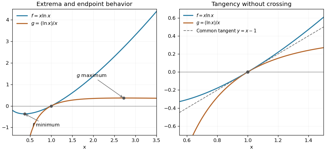
For , the derivatives are and . Its unique stationary point is the global minimum . For , changes from positive to negative at , giving the global maximum . Their endpoint limits areAn intersection requires , and on both factors vanish only at . There and , proving a common tangent line . In fact,because the two numerator factors always have the same sign. Thus the curves touch at without exchanging their order.

Past exam of the mathematics course of the year 1 of the natural sciences course of the University of Cambridge 2001 Paper 1 4 c Solution Created 2026-10-18 Updated 2026-10-20
The fundamental theorem of calculus and part (a) giveThe difference is constant in . Since , the constant is zero, provingThis is simply the chain rule integrated, with itself as the antiderivative of the square-root factor.
Past exam of the mathematics course of the year 1 of the natural sciences course of the University of Cambridge 2001 Paper 1 4 b Solution Created 2026-10-18 Updated 2026-10-20
Work first with , so the real integrands and their parameter derivatives are smooth on every finite amplitude interval. For the elliptic integral of the second kind,On the other hand, subtracting the integrands of the second-kind and first-kind elliptic integrals givesConsequentlyThis is the modulus derivative of the incomplete elliptic integral of the second kind. At its right-hand side has a removable limit zero, agreeing with . Both and here use amplitude and modulus ; differentiating with respect to the alternative parameter would give a different prefactor.
There are unlisted articles, also show them or only show them.