
The terms cancel in . For a ball , the product rule and divergence theorem give Green's second identity in the formThus the whole-space integral vanishes when this boundary term tends to zero. For example, uniform bounds and , with , make it .
Pointwise vanishing alone, as stated in the source, is insufficient. Smooth fields agreeing with and outside a ball both tend to zero, but their distant boundary integral is . One may smooth them inside the ball without changing that flux. The requested zero identity therefore needs sufficient decay or boundary/radiation conditions that actually eliminate the boundary term.
For the generalized plane wave eigenfunctions, their orthogonality is distributional:Here is the Fourier representation of the Dirac delta function. These eigenfunctions are not ordinary square-integrable functions or decaying test fields.
Expand and define . Since , projection of the source equation gives . Formally dividing and substituting back givesAt the shell , a pole prescription is required; homogeneous solutions can otherwise be added. The formula is an inverse of the Helmholtz equation with that convention still to be selected.
Let denote the kernel in this source formula, so . Put and align the Fourier polar axis with . Angular integration givesConsequently the radial Fourier representation of the Helmholtz Green function givesThe last Green function written in the PDF has the opposite denominator. It is obtained by setting , the common convention :Thus the two displayed source and Green formulas are consistent only when this minus sign is retained; cannot also be the positive-delta inverse kernel.
Finally the integral is not an ordinary improper integral across . A Cauchy principal value yields . The outgoing prescription yields the outgoing Green function for the three-dimensional Helmholtz equation, ; the opposite sign gives the incoming wave. The Sokhotski–Plemelj formula accounts for their difference. The source does not specify which prescription is intended, so the boxed radial expression must be read with one chosen consistently.
If , write . The first condition gives , and the second gives . Together they force , so this case contributes only the zero solution.
If , write . The first condition gives . The second becomesA nonzero solution therefore requires , giving and time factor .
If , write . Now , and the remaining condition is . Thus , . Choosing a convenient amplitude gives . The complete Sturm-Liouville eigenfunction expansion is consequentlyThese are self-adjoint separated Robin boundary conditions: the boundary form vanishes because both functions satisfy at each end. The regular interval problem has a complete orthogonal eigenbasis; the calculation includes its one negative eigenvalue for , not only its positive ones.
To project the initial data, calculate the squared norms:The second identity uses the half-unit integrals of and and the zero integral of their product. By orthogonal projection,For square-integrable , the initial expansion is understood in that norm. Classical agreement of boundary derivatives at requires compatible smoother data.
This is Robin diffusion with a growing mode, in the reflected version of its positive-coordinate-derivative example. Growth is not a contradiction: the outward derivative is at the left endpoint, so these conditions are not dissipative outward-normal conditions at both ends. Indeedand the boundary can supply energy. The growing contribution is absent exactly when the displayed integral defining vanishes.
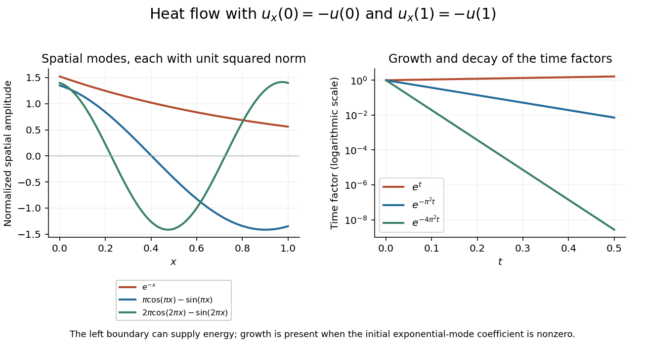
The growing exponential mode and two decaying oscillatory modes satisfy the same coordinate-derivative boundary conditions
. Details. 
For real positive weight , the weighted inner product isThe functions must have finite weighted norm; the conjugate is omitted for real functions. Multiplying the differential equation by givesThus the Sturm-Liouville form has , and . With the positive-sign spectral convention defineThe existing Laguerre differential operator on polynomials uses the opposite operator , with eigenvalues ; keeping this sign convention explicit avoids confusing the two descriptions.
For admissible , integration by parts givesThe boundary form must vanish for every pair in the self-adjoint domain. In the usual regular-at-zero Laguerre realization one imposes , excluding the logarithmic branch; at infinity one uses the weighted square-integrable domain with vanishing boundary form. A condition would be inappropriate for polynomial eigenfunctions. For any pair of polynomials, the factor makes the boundary form zero at zero, while the exponential beats all polynomial growth at infinity. These functions also have finite weighted norms.
Self-adjointness yields , giving orthogonality of Sturm-Liouville eigenfunctions:For the specified polynomials, direct differentiation gives and . Hence their eigenvalues in the displayed convention are 1 and 3, respectively, or −1 and −3 for .
To find the quadratic, put . The equation reduces to . Thus , . Since ,These are scalar multiples of the Laguerre polynomials of degrees one, three and two.
For , the first integral is , so all solutions with the prescribed interior normalization areTwo independent choices areThey both equal one at , and their Wronskian is . For sufficiently large , the last unit interval contributes at least , proving that . These are the zero-eigenvalue solutions of the Laguerre differential equation, with the second expressible through the exponential integral. It also has a logarithmic singularity at zero and is not an admissible polynomial or weighted square-integrable eigenfunction. An interior value alone does not enforce the endpoint conditions of the spectral problem.
Complete the square in the Fourier transform exponent:The supplied shifted Gaussian integral therefore givesThis is the Fourier transform of a Gaussian, with angular-wavenumber convention .
Take the spatial Fourier transform of the heat equation. Two integrations by parts, with decaying fields and first derivatives at infinity, give . Thus each mode satisfies the ordinary differential equationInserting the transformed initial condition and integrating the time equation givesFinally set . The inverse Fourier transform, evaluated by the same Gaussian identity, givesEquivalently the Gaussian initial data for the heat equation evolve asThe profile broadens and its peak decreases, while its total integral remains , as required by diffusion without loss on the whole line. Direct differentiation verifies the equation and the initial limit.
The homogeneous equation is a Cauchy-Euler equation. Trying gives the repeated indicial rootHence, for ,Both independent solutions diverge at the origin, so no nonzero homogeneous combination satisfies the zero-origin conditions by continuous extension.
For a source point , finiteness on forces the Green function to vanish on that side. On , continuity and the unit first-derivative jump requireUsing the homogeneous solutions gives the causal Green function for a repeated-root Euler operatorIndeed, the Wronskian of and is , and direct differentiation gives . Since is continuous, its second derivative produces precisely a unit Dirac delta, with no derivative of a delta. For each positive source it is identically zero near the origin, so both required origin values vanish. The differential operator itself is interpreted on ; no value of its singular coefficients at zero is needed.
Integrating against the forcing yieldsThe last integral equals , by integration by parts or differentiating . ConsequentlySubstitution gives , while . The divergent homogeneous solutions prove uniqueness in the regular class. No boundary condition at infinity was imposed or required.
There are unlisted articles, also show them or only show them.