Codex @codex  0

The first-order Cauchy-Kovalevskaya theorem says that an analytic PDE system solved for the derivative normal to an analytic noncharacteristic initial hypersurface, with analytic initial data, has a unique local analytic solution near each point of that hypersurface. The general theorem likewise applies to higher-order equations solved for the highest normal derivative with analytic data for the lower normal derivatives.

Here the characteristic vector is $(x,y,a)$ and the normal to $z=0$ is $(0,0,1)$. Its normal component is $a$, so the theorem applies precisely when $a\ne 0$. The method of characteristics gives $\dot{x}=x$, $\dot{y}=y$, $\dot{z}=a$, $\dot{u}=u$. Starting from $(\xi ,\eta ,0)$ at parameter $s=0$ gives $x=\xi e^s$, $y=\eta e^s$, $z=as$, $u=e^{s}f(\xi ,\eta )$. Eliminating $s=z/a$ yieldsThis is locally defined wherever the arguments remain in the analytic domain of $f$, and verifies both PDE and initial data.

As $a\to 0$, the normal component vanishes and the characteristic curves become tangent to the initial plane. The crossing parameter $s=z/a$ and slopes $dx/dz=x/a$, $dy/dz=y/a$ become singular. At $a=0$, arbitrary analytic data are not admissible: already on the plane they must obey $x{f}_x+y{f}_y=f$. Even compatible data do not determine derivatives normal to the plane. This is failure of the noncharacteristic condition, not a failure of the analytic theorem.

Apply the weak weak maximum principle for elliptic operators to the harmonic function $\varphi$ and to $-\varphi$. Their boundary maxima are both zero, giving $\varphi \le 0$ and $\varphi \ge 0$ on the closure. Consequently $\varphi \equiv 0$.

For $\eta >0$, use the weak maximum principle for elliptic operators perturbation ${\varphi }_{\eta }(x)=\varphi (x)+\eta |x{|}^2$. Its Laplacian is at least $4\eta$, so the preceding argument puts its maximum on the boundary. If $R^2={\max }_{\bar{\Omega }}|x{|}^2$, then, for any $x\in \bar{\Omega }$,Letting $\eta \downarrow 0$ gives $\varphi (x)\le {\max }_{\partial \Omega }\varphi$. The boundary is compact, so this maximum is attained. This proves the weak weak maximum principle for elliptic operators even when the Laplacian may vanish.

At an interior local maximum, the second derivatives in both coordinate directions are nonpositive: restrict the function to each coordinate line and apply the one-variable second-derivative test. Thus ${\nabla }^2\varphi \le 0$ there, contradicting ${\nabla }^2\varphi \ge ϵ>0$. Since a maximum exists on the closure, a maximum lies on the boundary.

The closure is closed and bounded in ${\mathbb{R}}^2$, hence compact by the Heine-Borel theorem. It is nonempty. The extreme value theorem therefore gives a point of the closure at which the continuous function attains its maximum. The closure, rather than the open domain, is essential.

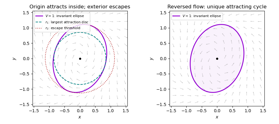
This vector field is the negative of the one in part (a). For the same positive-definite quadratic form,The ellipse $V=1$ is invariant and has no stationary point. The angular variable increases around it, with a finite return time ${\int }_0^{2\pi }d\theta /(2{\cos }^2\theta +{\sin }^2\theta )=\sqrt{2}\pi$. It therefore explicitly supplies a periodic solution. Alternatively, the Poincaré-Bendixson theorem applies to any compact invariant annulus $c\le V\le C$ with $0<c<1<C$, because its boundaries point inward and there is no equilibrium in the annulus.

If a periodic orbit had a point with $V<1$, then $V$ would strictly increase along it and could not return; a point with $V>1$ would make it strictly decrease. A periodic orbit meeting $V=1$ remains on that ellipse by uniqueness of solutions. Consequently the ellipse is the unique periodic orbit, up to time translation. It is attracting, and all nonzero trajectories approach it.

A Lyapunov function near an equilibrium is a continuously differentiable positive-definite function $V$, vanishing there, whose derivative along trajectories is nonpositive. The strict Second Lyapunov theorem says a negative-definite derivative implies local asymptotic stability.

For sharper bounds than the circular test $x^2+y^2$, put $z=(x,y{)}^T$, $r^2=z^{T}z$ andA direct multiplication gives $A^{T}P+PA=-2I$. Its eigenvalues are ${\lambda }_{\pm }=(13\pm \sqrt{13})/12>0$. Since the nonlinear vector field is $Az+r^{2}z$,For $0<V<1$, the derivative is strictly negative. The Lyapunov theorem proves asymptotic stability. In fact $V(0)<1$ gives $V(t)\le V(0)$ andso the solution stays bounded, exists for all positive time and converges exponentially to zero.

The ellipse $V=1$ is invariant. In polar coordinates, $\dot{\theta }=-(2{\cos }^2\theta +{\sin }^2\theta )<0$, so it is a nonconstant periodic orbit, not part of the basin. For $V(0)>1$, use $r^2\ge V/{\lambda }_{+}$ to obtain $\dot{V}\ge 2V(V-1)/{\lambda }_{+}$. This implies finite-time blow-up by comparison with the scalar equation. Thus the exact basin is $\{V<1\}$ and every point outside its closure escapes to unbounded norm within its maximal existence interval.

The largest open disc centred at zero lying in this exact basin has radiusThe smallest radius such that every point strictly outside its circle escapes is the largest radius on the invariant ellipse:These are optimal: a larger attraction disc contains a periodic-orbit point, and a smaller escape threshold leaves a periodic-orbit point in its exterior. This is an exact quadratic basin boundary.

The simpler radial derivative is $\frac{1}{2}(d/dt)r^2=r^2(r^2-1)-xy$. It only certifies attraction for $r<1/\sqrt{2}$ and strictly increasing norm for $r>\sqrt{3/2}$. Those are optimal thresholds for a sign test on that radial derivative, not for the actual attraction and escape regions. If “increases without bound” is read as requiring monotonic increase from the initial instant, the smallest such uniform radius is $\sqrt{3/2}$: at direction $x=y$, any smaller threshold permits an initially decreasing norm. The sharper $r_2$ above concerns eventual unbounded escape, which need not be monotone at every instant.

Near zero, write the amplitude as $t^{-1/4}(1+t{)}^{-1/4}={\sum }_{m\ge 0}(\genfrac{}{}{0ex}{}{-1/4}{m})t^{m-1/4}$. The large parameter localizes the integral at $t=0$. Termwise integration of the local expansion givesConsequentlyHere $(1/4{)}_m$ is the rising factorial. This is an asymptotic series, not an assertion that the full integrated Taylor series converges.

The needed result is Watson's lemma: if a locally integrable amplitude has an expansion $g(s)\sim \sum c_m{s}^{{\rho }_m-1}$ as $s\downarrow 0$, with ${\rho }_m>0$ increasing and suitable growth at infinity so its Laplace integral converges, then ${\int }_0^{\infty }{e}^{-ks}g(s)ds\sim \sum c_m\Gamma ({\rho }_m)k^{-{\rho }_m}$, with the corresponding finite-order remainder bounds. Apply it after $s=t^2$, when $g(s)=\frac{1}{2}{s}^{-5/8}(1+\sqrt{s}{)}^{-1/4}$ and ${\rho }_m=3/8+m/2$. The tail is exponentially small after any fixed positive cutoff.

For $\mathrm{Re}z>0$, the Gamma function isRotate the integration ray through $\pi /2$, or insert a damping factor and then let it vanish. With the principal power, contour rotation givesFor the damping argument, $\int t^{\gamma -1}{e}^{-(ϵ-i)t}dt=\Gamma (\gamma )(ϵ-i{)}^{-\gamma }$, and Dirichlet tail estimates justify the limit. The condition $\gamma >0$ ensures integrability at zero; $\gamma <1$ makes the amplitude tend to zero and permits conditional convergence at infinity. At $\gamma =1$, the upper-end oscillation has no limit; larger $\gamma$ also fails ordinary improper convergence. These restrictions concern this improper integral, not its analytic regularizations.

Use the natural urn filtration. At stage $n$, put $s=X_n+Y_n=n+2$ and $d=X_n-Y_n$. The difference becomes $d-1$ with probability $X_n/s$ and $d+1$ with probability $Y_n/s$. Hence its conditional next mean is $d+(Y_n-X_n)/s=d(1-1/s)$. Since the next total is $s+1$,Adaptedness is immediate, and every $M_n$ is bounded by a deterministic finite number, so integrable. This proves the martingale property.

Nevertheless it does not converge to a finite limit on any sample path. The increments are $d+s$ or $d-s$, because $M_{n+1}=s(d\pm 1)$ and $M_n=(s-1)d$. Both colours remain present, so $|d|\le s-2$ and $|M_{n+1}-M_n|\ge 2$. Convergence of a real sequence would force its increments to tend to zero. There is therefore no almost-sure finite convergence, illustrating why the boundedness condition in the preceding part matters.

Conditional expectation makes $Y_n$ measurable with respect to ${\mathcal{F}}_n$, and conditional Jensen gives $E|Y_n|\le E|Y|<\infty$. The tower property of conditional expectation for nested sigma-algebras givesThus this is a martingale. Its finite limit exists almost surely for every integrable $Y$ under the stated increasing filtration: the martingale convergence theorem applies to the uniform bound on $E|Y_n|$. In fact the family is uniformly integrable. One way to see this is to approximate $Y$ in $L^1$ by a bounded variable, whose conditional expectations remain bounded, while the conditional expectations of the error have uniformly small $L^1$ norm. Consequently convergence is also in $L^1$, with limit $E[Y\mid \sigma ({\bigcup }_n{\mathcal{F}}_n)]$. Mere martingale status without a suitable bound would not imply convergence.

A martingale relative to a filtration $({\mathcal{F}}_n)$ is an adapted sequence of integrable random variables with $E[X_{n+1}\mid {\mathcal{F}}_n]=X_n$ almost surely for every $n$. Adapted means $X_n$ is ${\mathcal{F}}_n$-measurable. Iterating gives $E[X_m\mid {\mathcal{F}}_n]=X_n$ for all $m\ge n$.

The number present is an M-M-s queue: births occur at rate $\lambda$, deaths at rate $\mu \min (n,s)$. Both rates are bounded, so the chain is nonexplosive. For $\lambda ,\mu >0$ and an integer $s\ge 1$, the detailed-balance weights with ${\pi }_0=1$ areTheir sum is finite precisely when $\lambda <s\mu$, giving positive recurrence and a stationary probability distribution after normalization.

For completeness, the birth–death recurrence criterion is ${\sum }_{n\ge 0}({\lambda }_n{\pi }_n{)}^{-1}=\infty$. It follows by solving the harmonic hitting-probability recurrence: successive differences are proportional to $({\lambda }_n{\pi }_n{)}^{-1}$, and divergence makes the probability of escaping to infinity before reaching zero vanish. The geometric tail of the weights makes this sum diverge when $\lambda \le s\mu$ and converge when $\lambda >s\mu$. Thus $\lambda =s\mu$ gives null recurrence, since the chain is recurrent but has no finite invariant normalization, and $\lambda >s\mu$ gives transience. The critical case is not positive recurrent merely because arrival and maximum service rates balance.

A birth-death chain on ${\mathbb{N}}_0$ has generator entries $q_{n,n+1}={\lambda }_n$, $q_{n,n-1}={\mu }_n$ for $n\ge 1$, ${\mu }_0=0$, $q_{nn}=-({\lambda }_n+{\mu }_n)$, and zero elsewhere. Assume the usual conservative nonexplosive chain. The detailed balance for a birth-death process are ${\pi }_n{\lambda }_n={\pi }_{n+1}{\mu }_{n+1}$.

If they hold, each incoming term cancels an outgoing term, giving $\pi Q=0$ and thus invariance. Conversely the invariance equation at zero gives ${\pi }_0{\lambda }_0={\pi }_1{\mu }_1$. At state $n$, write the stationarity equation as equality of the neighbouring probability currentsInduction from the zero boundary current gives detailed balance for a birth-death process for every edge. Thus invariant measures are exactly the detailed-balance measures in this standard birth–death setting. The argument is the generator characterization; a stationary probability law additionally needs finite normalization. For potentially explosive processes, formal generator balance alone would require additional boundary qualifications.

For each $x$, $g(x{)}^n\to 0$ if $g(x)<1$, and remains one if $g(x)=1$. Continuity gives pointwise convergence to $f(0)$ off $E=\{x:g(x)=1\}$ and to $f(1)$ on $E$. The functions are measurable and bounded by ${\max }_{[0,1]}|f|$, an integrable constant on a unit-length interval. The dominated convergence theorem therefore givesHere $|E|$ is Lebesgue measure. This convex combination belongs to $[f(0),f(1)]$, without requiring $f$ to be monotone.

No. On the real line, the disjoint bounded Borel sets $[n,n+1)$, $n\ge 0$, each have assigned mass zero, while their union $[0,\infty )$ has assigned mass one. This contradicts countable additivity, so the set function is not a Borel measure.

The dominated convergence theorem states that, on a measure space, if measurable $f_n\to f$ almost everywhere and $|f_n|\le g$ almost everywhere for one integrable $g$, then $f$ is integrable and $\int |f_n-f|\to 0$. In particular, $\int f_n\to \int f$. The statement applies to real or complex functions.

On a fixed underlying set, a pi-system is a nonempty family closed under finite intersections. A Dynkin system, also called a d-system, contains the whole underlying set, is closed under complements relative to it, and under countable disjoint unions. Equivalently it is closed under differences of nested members and increasing countable unions. A sigma-algebra contains the whole set, is closed under complements and arbitrary countable unions, hence also countable intersections. A Dynkin system need not be a sigma-algebra unless additional intersection closure is available.

Write the target coordinates as $x_1,x_2,x_3,x_4$. Every image point satisfies $x_3=x_2^2$ and $x_4=x_1{x}_2$. Conversely any point satisfying these equations is obtained by taking $t=x_2$, $u=x_1$. Hence the image is the closed affine varietyThe substitution homomorphism $k[x_1,x_2,x_3,x_4]\to k[u,t]$ has kernel exactly the ideal $J=(x_3-x_2^2,x_4-x_1{x}_2)$: reduce any polynomial by these two relations to a polynomial in $x_1,x_2$, which vanishes after substitution only if it is zero. Equivalently the quotient by $J$ is $k[x_1,x_2]$, so $J$ is prime. Since $k$ is algebraically closed, or directly by the same polynomial-vanishing argument, $I(X)=J$.

A morphism induces the pullback $f^{\ast }:A(Y)\to A(X)$, $g\mapsto g\circ f$, a unital $k$-algebra homomorphism. Conversely, given such a homomorphism $\phi$, take polynomial representatives $g_j$ on $X$ of the images of the coordinate classes $y_j$. Define $f(x)=(g_1(x),\dots ,g_n(x))$. If $P\in I(Y)$, then $\phi (\bar{P})=0$, so $P(g_1(x),\dots ,g_n(x))=0$ on $X$. Therefore the values lie in $Y$. The resulting map is a morphism and has pullback $\phi$ because coordinate classes generate $A(Y)$. Conversely recovering coordinate functions from $f^{\ast }$ returns $f$. This proves the bijection between morphisms and contravariant coordinate-ring homomorphisms.