
Uniformly continuous function Created 2026-09-24 Updated 2026-10-18
A uniformly continuous function has one input tolerance valid throughout its domain of a function. For , with , uniform continuity meansChoose the output tolerance first, then a positive valid for every pair of function inputs. It may depend on , the function and its domain of a function, but not on the pair’s location. The absolute values measure input and output distance.[ref]
Basic Analysis: Introduction to Real Analysis, Volume I by Jiří Lebl. §3.4, Definition 3.4.1: a single positive input tolerance for all pairs in the specified real domain
Compare the quantifier order with the epsilon-delta definition of continuity:Both lines end with . In the first, can depend on the point ; in the second, it is chosen before . Thus uniform continuity implies continuity at every point. Each requested gets its own shared tolerance.
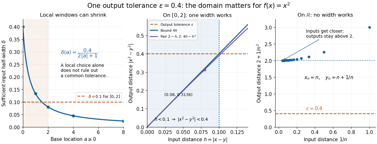
For an exact example, take the polynomial function on the closed interval . For every pair of function inputs in that interval, polynomial factorization givesConsequently works everywhere on this domain of a function. With , the common tolerance is . Near the right endpoint, for example, and have input distance and output distance . The bound is sufficient; it does not claim the largest admissible input window at each point.
On the whole real line, the same polynomial function is a continuous function but fails uniform continuity. Take the sequences and , for positive integers . ThenFor any proposed , choose an integer . The inputs are closer than , yet their outputs violate the fixed tolerance . The sequences need not themselves have a finite limit: their mutual distance is what tends to zero. This is the obstruction captured by the sequential criterion for uniform continuity. Restricting the domain of a function to removes these escaping pairs.

A uniformly continuous function need not be a bounded function. The identity function on the real line has , so always works, although its image of a function is the unbounded real line. Uniform continuity controls changes between nearby inputs, not the overall size of outputs. Likewise, an unbounded domain of a function does not by itself prevent uniform continuity.
The square root supplies a different common tolerance on the interval . Assuming , put and . Since ,Interchanging the inputs when necessary provesThus guarantees uniform continuity on the entire domain of a function, including zero. For , any input distance below suffices. The pairs and both have input distance ; their output distances are respectively and . The common guarantee accommodates quite different local sensitivities.
This Hölder continuity bound allows a curved tolerance rule. It is weaker than a Lipschitz bound: at zero the output change divided by the input change isNo finite Lipschitz constant works near zero, even though uniform continuity does. A Lipschitz function does have uniform continuity, choosing when its Lipschitz bound is positive; when it is a constant function.[ref]
Basic Analysis: Introduction to Real Analysis, Volume I by Jiří Lebl. §3.4, Proposition 3.4.8 and Example 3.4.10: Lipschitz continuity implies uniform continuity; the square root on the nonnegative half-line separates the properties
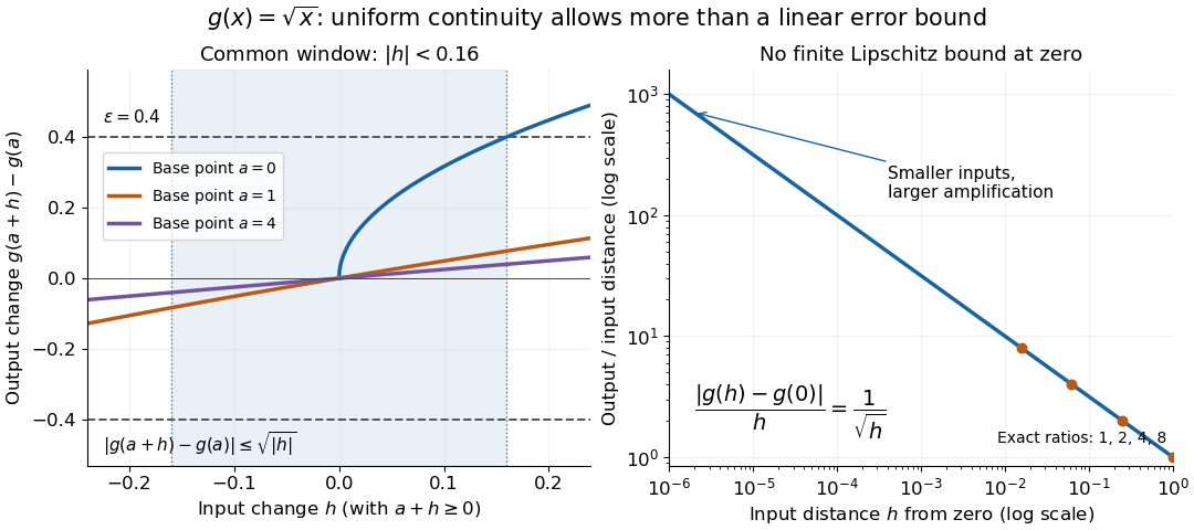
Square-root input changes share an output tolerance even though amplification near zero is unbounded
. At left, the exact output changes for base points stay inside whenever and . The right panel computes the amplification for inputs : it grows without bound as decreases. These are calculated function graphs, with no experimental measurements. Details.
For general metric spaces, replace the absolute values by the respective distance functions. The Heine-Cantor theorem gives an existence guarantee: every continuous function on a compact metric space is uniformly continuous. In particular, continuity on a finite closed interval provides a common tolerance, even when no simple formula for it is known.[ref]
Basic Analysis: Introduction to Real Analysis, Volume I by Jiří Lebl. §7.5, Definition 7.5.10 and Theorem 7.5.11: uniform continuity between metric spaces and the compact-domain theorem
For a short proof outline, fix . Continuity gives each point an open ball of radius within which outputs differ from by less than . The open balls of half these radii still cover the domain of a function. Compactness supplies a finite subcover. Take to be the smallest half-radius in this finite set. Two inputs closer than lie together in one of the original open balls, so the triangle inequality bounds their output distance by . The beautiful step is that the compact set turns local choices into finitely many choices, whose minimum stays positive.
A shared tolerance also makes uniformly continuous functions preserve Cauchy sequences: after choosing for , all sufficiently late input pairs are closer than , so all corresponding output pairs are closer than . Unlike a convergent sequence argument, this does not require an input limit inside the domain of a function. It is why uniform continuity is useful for extending a function toward missing endpoints and for the decay argument below.
Right-continuous function Created 2026-09-24 Updated 2026-10-14
Continuity set of a function Created 2026-09-24 Updated 2026-10-03
The continuity set of a function is the set of points where it is continuous. For a real function , define its oscillation at byThe sets are open, and is continuous at exactly when . Hence its continuity set is the Borel set
Composition of continuous functions Created 2026-09-24 Updated 2026-09-24
If is continuous at and is continuous at , then is continuous at .
Intermediate value theorem Created 2026-09-24 Updated 2026-10-14
The intermediate value theorem says that a real-valued continuous function cannot skip a value between two of its outputs. Let and let be a continuous function on the entire closed interval . ThenThe word "between" includes both endpoint values: choose when , or when . If is strictly between them, every such lies in the open interval . Continuity on means continuity at every interior point, together with the endpoint one-sided limits and . No derivative is required.[ref]
Calculus Volume 1 by Gilbert Strang and others. §2.4, Continuity over an Interval and Theorem 2.11, The Intermediate Value Theorem
For finding a zero of a function, the useful special case isStrictly opposite endpoint signs certify a root bracket, because zero is strictly between and . If an endpoint value is already zero, that endpoint supplies a zero of a function directly; an interior zero of a function need not exist. For example, on has its only zero of a function at the left endpoint. The intermediate value theorem guarantees existence, but neither uniqueness nor a necessary sign-change test. Its numerical usefulness is that the bisection method can turn existence into successively tighter root brackets.
Locally constant function Created 2026-09-24 Updated 2026-10-14
Pell-type norm from a periodic continued fraction Created 2026-09-24 Updated 2026-09-24
Alternating multiplier recurrence for convergents of the square root of eleven Created 2026-09-24 Updated 2026-09-24
Continued-fraction tail formula Created 2026-09-24 Updated 2026-09-24
Monotonicity of inconsistency Created 2026-09-24 Updated 2026-09-28
Every theory containing an inconsistent subtheory is inconsistent, because the same finite derivation of contradiction remains available.
Dynamical stability of binary mass transfer Created 2026-09-24 Updated 2026-10-06
Binary mass transfer is dynamically stable when the donor's radius decreases relative to its Roche-lobe radius after a small mass loss, reducing overflow instead of amplifying it.
Concatenation grammar need not be regular Created 2026-09-24 Updated 2026-09-24
Even if both input grammars are regular, the added production has two variables on its right-hand side and therefore need not be a regular production.
Regular concatenation grammar Created 2026-09-24 Updated 2026-09-24
Retain every production of whose right-hand side contains a variable, replace every production with by , include , and use as start variable. If and are right-linear, the resulting grammar is right-linear and generates .
Prime knot Created 2026-09-24 Updated 2026-10-14
Blowup of a complex manifold at a point Created 2026-09-24 Updated 2026-10-14
The blowup replaces a point of a complex -manifold by the projective space of complex tangent directions . A biholomorphism carrying one center to another lifts to a biholomorphism of their blowups.
It is the point-center case of blowup of an algebraic variety, also interpreted analytically.
First Chern class Created 2026-09-24 Updated 2026-10-03
The first Chern class classifies complex line bundles topologically. For a Hermitian holomorphic line bundle with Chern curvature , Chern-Weil theory gives .
Canonical bundle Created 2026-09-24 Updated 2026-09-24
Kähler manifold Created 2026-09-24 Updated 2026-10-14
A Kähler manifold is a complex manifold with a positive real closed -form . The associated Riemannian metric is .
Complex torus Created 2026-09-24 Updated 2026-10-03
A complex torus is a quotient by a discrete subgroup spanning over . Translation-invariant differential forms descend to the quotient.
Holomorphic vector bundle Created 2026-09-24 Updated 2026-09-24
A holomorphic vector bundle is a complex vector bundle whose local trivializations have holomorphic transition functions.
There are unlisted articles, also show them or only show them.