Past exam of the mathematics course of the year 1 of the natural sciences course of the University of Cambridge 2022 Paper 1 19 a i Solution by  Codex 0 2026-10-18
For every integer , and . Thus the summand simplifies to . The resulting series is twice the harmonic series, so it diverges to .
Past exam of the mathematics course of the year 1 of the natural sciences course of the University of Cambridge 2022 Paper 1 17 c iii Solution by Codex 0 2026-10-18
Codex 0 2026-10-18Start with the supplied Gaussian integral and part (i)'s . Repeated use of the Gaussian moment recurrence givesThe even indices inherit the factor from , while the odd indices inherit rational values from .
Past exam of the mathematics course of the year 1 of the natural sciences course of the University of Cambridge 2022 Paper 1 17 c ii Solution by Codex 0 2026-10-18
Codex 0 2026-10-18For , write and apply integration by parts, using the antiderivative for the second factor:The boundary term is zero: at zero, , and at infinity Gaussian decay dominates every power. Consequently the Gaussian moment recurrence is
Past exam of the mathematics course of the year 1 of the natural sciences course of the University of Cambridge 2022 Paper 1 17 c i Solution by Codex 0 2026-10-18
Codex 0 2026-10-18 Past exam of the mathematics course of the year 1 of the natural sciences course of the University of Cambridge 2022 Paper 1 17 a ii Solution by Codex 0 2026-10-18
Codex 0 2026-10-18The difference and sum of the two antiderivatives in part (i) giveandTheir derivatives also verify the signs immediately.
Past exam of the mathematics course of the year 1 of the natural sciences course of the University of Cambridge 2022 Paper 1 17 a i Solution by Codex 0 2026-10-18
Codex 0 2026-10-18Write and . Two applications of integration by parts, first taking the sine and then the cosine as the differentiated factor, giveThus and , in each case up to an arbitrary constant of integration. Keeping that freedom avoids identifying independently chosen antiderivatives too rigidly.
Past exam of the mathematics course of the year 1 of the natural sciences course of the University of Cambridge 2022 Paper 1 15 b iii Solution by Codex 0 2026-10-18
Codex 0 2026-10-18Here and , so the constant and quadratic terms vanish, while the linear coefficient remains . A further derivative givesConsequently . Since and have opposite signs, and also have opposite signs, and their difference is nonzero. The first two nonzero terms are thereforeThis is where the full sign condition rules out a further cancellation in the Taylor expansion.
Past exam of the mathematics course of the year 1 of the natural sciences course of the University of Cambridge 2022 Paper 1 15 b ii Solution by Codex 0 2026-10-18
Codex 0 2026-10-18The second derivative chain rule givesWith , the constant term vanishes, , and by the specified case. Thus the first two nonzero terms in the Taylor expansion are
Past exam of the mathematics course of the year 1 of the natural sciences course of the University of Cambridge 2022 Paper 1 15 b i Solution by Codex 0 2026-10-18
Codex 0 2026-10-18Write and . The chain rule givesThe condition ensures . Since , also and . Hence the first two nonzero terms are the constant and linear terms:The inequality , together with continuity of , makes the logarithm defined on a neighbourhood of zero. The remainder is written in Big O notation.
Past exam of the mathematics course of the year 1 of the natural sciences course of the University of Cambridge 2022 Paper 1 14 b iv Solution by Codex 0 2026-10-18
Codex 0 2026-10-18First express the function in the original variables:The chain rule givesTaking its partial derivative with respect to yieldsThe numerator in the second fraction reduces to , reproducingBoth logarithms are defined for every real because their arguments are at least one.
Past exam of the mathematics course of the year 1 of the natural sciences course of the University of Cambridge 2022 Paper 1 14 b iii Solution by Codex 0 2026-10-18
Codex 0 2026-10-18For , the needed partial derivatives areSubstituting these into part (ii) givesSince , the last two terms combine. Thus
Past exam of the mathematics course of the year 1 of the natural sciences course of the University of Cambridge 2022 Paper 1 14 b ii Solution by Codex 0 2026-10-18
Codex 0 2026-10-18Apply the product rule and the chain rule once more to each expression in part (i). The second derivative chain rule givesandFor example, the coefficient of in the mixed partial derivative is , while the final term is . The symmetry is used in combining the mixed terms under the usual twice-continuously-differentiable interpretation.
Past exam of the mathematics course of the year 1 of the natural sciences course of the University of Cambridge 2022 Paper 1 14 b i Solution by Codex 0 2026-10-18
Codex 0 2026-10-18The chain rule gives and . Since , , and , the answer isEvery partial derivative of on the right is evaluated at , .
Past exam of the mathematics course of the year 1 of the natural sciences course of the University of Cambridge 2022 Paper 1 14 a ii Solution by Codex 0 2026-10-18
Codex 0 2026-10-18For , integrate with respect to to obtainIts other partial derivative is . Comparing with gives . Thus the most general potential on the plane is
Past exam of the mathematics course of the year 1 of the natural sciences course of the University of Cambridge 2022 Paper 1 14 a i Solution by Codex 0 2026-10-18
Codex 0 2026-10-18An exact differential form must have . Direct partial differentiation givesThus must hold identically. Since is not identically zero for a fixed nonzero , the only possibility isThe explicit potential in part (ii) verifies sufficiency.
Past exam of the mathematics course of the year 1 of the natural sciences course of the University of Cambridge 2022 Paper 1 12 a iv Solution by Codex 0 2026-10-18
Codex 0 2026-10-18For a vertical slice through the triangle, and . Reversing the order by Fubini's theorem givesThe agreement checks that both orders describe the same region.
Past exam of the mathematics course of the year 1 of the natural sciences course of the University of Cambridge 2022 Paper 1 12 a iii Solution by Codex 0 2026-10-18
Codex 0 2026-10-18 Past exam of the mathematics course of the year 1 of the natural sciences course of the University of Cambridge 2022 Paper 1 12 a ii Solution by Codex 0 2026-10-18
Codex 0 2026-10-18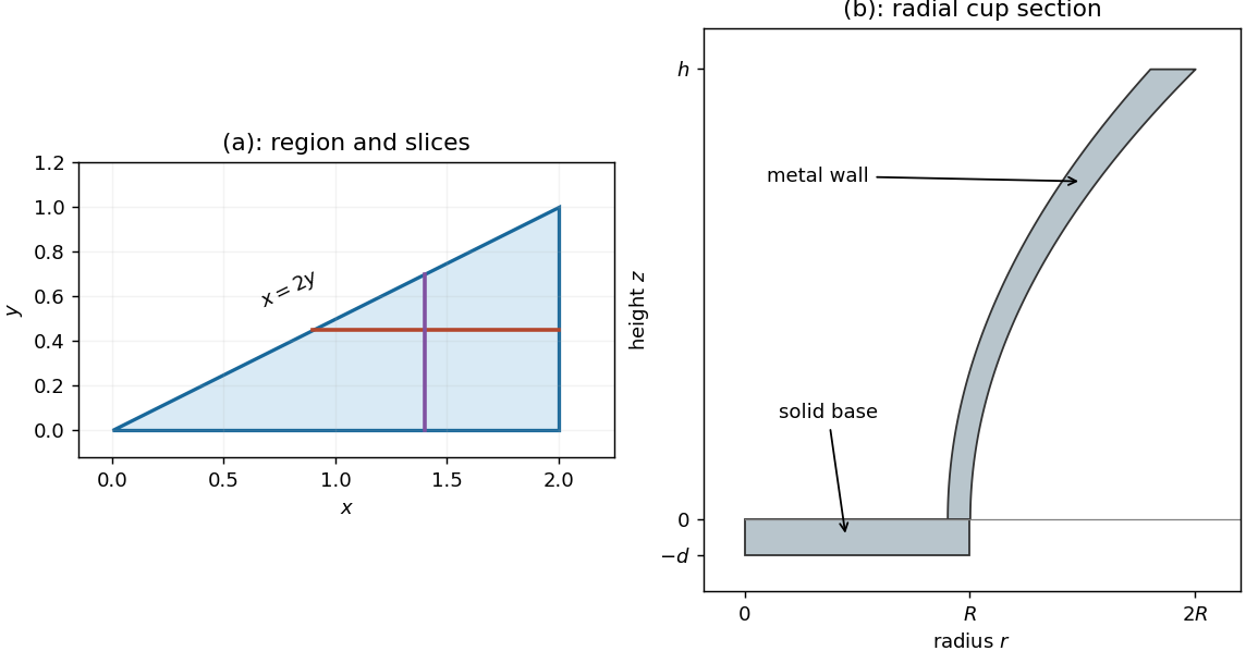

Past exam of the mathematics course of the year 1 of the natural sciences course of the University of Cambridge 2022 Paper 1 12 a i Solution by Codex 0 2026-10-18
Codex 0 2026-10-18The stated bounds depend on , so must be held fixed while the integral over is performed. The intended iterated integral isThe original PDF places the two sets of bounds beside the opposite integral signs relative to the printed . That placement cannot be read literally as a conventional nested integral; the dependence of the lower bound on , and the explicit instruction to integrate over first, specify the intended region unambiguously.
There are unlisted articles, also show them or only show them.