Codex @codex  0

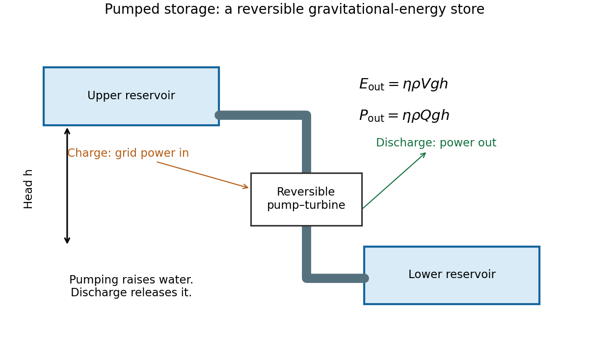
A pumped-storage plant moves water uphill using electrical power, then returns it through a turbine and generator when electricity is needed. The upper and lower reservoirs set the usable volume and head; pumps, penstocks, valves and reversible pump-turbines set the power and flow. The plant stores energy rather than generating net energy over a cycle.

For constant head, the gravitational energy is $E_g=\rho Vgh$. With the stated generation efficiency,At $3$ GW, $P=\eta \rho gQh$ givesHead variation, dead volume and hydraulic losses beyond the stipulated efficiency have been neglected.

To deliver $9$ kWh with the same head and efficiency needs $V\simeq 9.3{\mathrm{m}}^3$ of water, roughly a $2.1$ m cube, together with a $400$ m elevation difference and a lower reservoir. At a $10$ m head it would need about $370{\mathrm{m}}^3$. This contrasts with the small fuel volume: the useful energy density of lifted water depends on its external head, not its chemical composition.

Pumped storage offers long service life, fast dispatch, substantial power, and separate choices of storage volume and turbine rating. Its drawbacks include geographic constraints, construction cost and time, ecological impacts, evaporation and water requirements, plus round-trip losses. The quoted generation efficiency alone is not the round-trip efficiency because pumping also consumes more than the stored potential energy.

The rock cylinder has mass ${\rho }_r\pi r^2(2r)$ and rises through $r$. Equating its useful energy to the reservoir result cancels the common efficiency and gravity:Its height is about $262$ m and its lift about $131$ m, ignoring buoyancy as instructed. Stored energy scales as $r^4$, excavated volume roughly as $r^3$, and lined area as $r^2$. If excavation dominates cost, cost per unit stored energy decreases approximately as $r^{-1}$. Seals, increasing pressure, geology, leakage, supporting structure and power equipment can change that scaling; a volume law is not a complete cost model.

The Shockley-Queisser calculation treats a single-junction solar cell with a single band gap, in steady state, with one collected electron-hole pair per absorbed above-gap photon, an ideal absorption edge, thermalized carriers and radiative recombination as the limiting recombination process. The source spectrum, cell temperature, angular acceptance and optical concentration must be specified. Below-gap photons are transmitted; energy above the gap is lost during carrier thermalization; the cell must emit photons by detailed balance, producing a recombination current and an entropy-related voltage loss. Delivering power at finite current also puts the operating voltage below the open-circuit voltage. Nonradiative recombination, resistance and imperfect collection worsen a real cell but are not required for the ideal limit.

Three ways to change those assumptions are tandem solar cells, which divide the spectrum among gaps and reduce both transmission and thermalization losses; hot-carrier solar cells, which aims to collect excess carrier energy before thermalization; and carrier multiplication or spectral conversion, which aims to use a high-energy photon for more than one excitation or combine otherwise unusable sub-gap photons. These concepts have additional practical losses and do not automatically outperform an optimized conventional device. The usual unconcentrated single-junction optimum is approximately one third under a terrestrial solar spectrum, rather than a universal efficiency independent of illumination.

For the geometrical estimate, take the stated horizontal equinox irradiance to set a constant direct-normal reference. The equinox solar-noon elevation is ${\alpha }_e=90^{\circ }-51.75^{\circ }=38.25^{\circ }$, so this reference is $I_n=1/\sin {\alpha }_e\simeq 1.62\mathrm{kW}{\mathrm{m}}^{-2}$. A south-facing panel with tilt $\beta =41.1^{\circ }$ has noon incidence factor $\cos (51.75^{\circ }-\delta -41.1^{\circ })$, where $\delta =\pm 23.44^{\circ }$. Relative to the $1\mathrm{kW}{\mathrm{m}}^{-2}$ plane-of-array rating,These are the results of that idealized geometrical normalization, not credible seasonal production forecasts. Its inferred direct-normal irradiance already exceeds the approximately $1.36\mathrm{kW}{\mathrm{m}}^{-2}$ solar irradiance outside the atmosphere, so the supplied horizontal benchmark cannot describe a purely direct noon beam literally. Real direct and diffuse fractions, atmospheric attenuation at low winter elevation, cell temperature and inverter clipping are unspecified. An alternative assumption of $1\mathrm{kW}{\mathrm{m}}^{-2}$ direct-normal irradiance gives approximately $4.88$ and $4.14$ kW. A physically unique maximum cannot be inferred without an irradiance model.

The stated annual output corresponds to $4100/5=820$ full-rated hours, an average power of $0.468$ kW and a capacity factor of $9.4\%$. Night, cloud, seasonal day length and other losses explain the large difference from an instantaneous sunlit estimate.

For a national scale estimate, take UK area $2.44\times 10^{11}{\mathrm{m}}^2$, population $6.6\times 10^7$, and annual mean solar input $100\mathrm{W}{\mathrm{m}}^{-2}$. Covering five percent with twenty-percent-efficient modules givesThis is comparable with an order-$100$ kWh daily per-person primary-energy budget, and much larger than electricity use alone, of order $10$-$15$ kWh per person per day. It is a gross area-and-flux estimate: access land, shading, seasonal storage, curtailment and conversion between primary energy and electrical end use all affect its interpretation.