Codex @codex  0

Normalize $v_K$ by $v_K({\pi }_K)=1$ and put $v_K(0)=+\infty$. Write $f(X)={\sum }_{j=0}^d{a}_j{X}^j$, with $a_d=1$ and $a_0\ne 0$. In the usual coefficient-exponent convention, the Newton polygon $N_K(f)$ is the lower boundary of the convex hull of the upward vertical rays starting atIt runs from $(0,v_K(a_0))$ to $(d,0)$, with nondecreasing slopes from left to right. Zero coefficients contribute no finite point. Equivalently it is the largest convex piecewise-linear function lying below all these coefficient points.

The Newton polygon root valuation theorem says that a segment of slope $s$ and horizontal length $r$ accounts for exactly $r$ roots of valuation $-s$, counted with multiplicity, using the extended valuation on an algebraic closure. The nonzero constant coefficient excludes a zero root.

For a short justification, use the weighted Gauss valuation $w_t(P)={\min }_j(v(c_j)+jt)$ for $P=\sum c_j{X}^j$. It is multiplicative: after scaling $X$ by an element of valuation $t$ in a valued extension, the initial nonzero residue polynomials multiply without vanishing. Rational $t$ suffice. Factoring a monic polynomial into linear factors gives $w_t(f)={\sum }_r\min (t,v(r))$. This supporting-line function changes derivative at precisely the root valuations; its derivative drops count their multiplicities. Supporting lines to the lower polygon have slope $-t$, proving the sign and horizontal-length assertion.

Slope convention for part (b). Reflecting the horizontal axis, by plotting $(d-j,v_K(a_j))$, produces the reflected Newton polygon convention; its slopes are the root valuations themselves. Part (b)'s wording with $m$ instead of $-m$ is correct under this positive-root-valuation convention. The proof below gives both forms explicitly, so the result does not depend on silently changing the sign.

A finite field extension $L/K$ is a separable field extension if every element of $L$ has a minimal polynomial over $K$ with distinct roots in an algebraic closure. The primitive element theorem says that a finite separable field extension $L/K$ is $K(\alpha )$ for some $\alpha \in L$.

If $K$ is finite, then so is $L$. The multiplicative group of a finite field is cyclic, so a generator of $L^{\times }$ generates $L$ as a field. To justify the group fact, a finite subgroup of a field's multiplicative group is cyclic: in a finite abelian group its exponent is attained as an element order, while the polynomial root bound forces its size to be at most that exponent.

If $K$ is infinite, first consider $L=K(a,b)$. The minimal polynomials of $a$ and $b$ have distinct roots $a_i,b_j$ in an algebraic closure. Choose $c\in K$, $c\ne 0$, avoiding the finitely many values for which $a_i+c{b}_j=a+cb$ for a pair other than $(a,b)$. Set $\alpha =a+cb$. Over $K(\alpha )$, the polynomials $f(T)$ and $g((\alpha -T)/c)$ have precisely one common root, $a$. Their monic greatest common divisor is therefore $T-a$, so $a\in K(\alpha )$ and $b=(\alpha -a)/c\in K(\alpha )$. Thus $K(a,b)=K(\alpha )$. Induct over finitely many generators of the finite separable field extension. This proves every finite separable extension is simple.

Write $q=p^r$, where $p=\mathrm{char}K$. Forthe derivative isso $h$ is a separable polynomial and all its roots in its splitting field $L$ are distinct.

Let $R$ be the set of these roots. The Frobenius endomorphism and the identitiesshow that $R$ is closed under addition and multiplication. It is also closed under additive inverses and, for $x\ne 0$, inversion. Thus $R$ is a finite field. Since $h$ splits into $q^n$ distinct linear factors, $|R|=q^n$. The field generated by all roots is therefore $R$ itself, so $L=R$ andHence the polynomial characterization of a finite field gives

Now let $f\in K[X]$ be irreducible of degree $n$, and let $\alpha$ be a root in an algebraic closure. The minimal polynomial of an algebraic element givesso $K(\alpha )$ has $q^n$ elements. Its nonzero elements form a finite group under multiplication, of order $q^n-1$; hence ${\alpha }^{q^n}=\alpha$. Therefore $\alpha$ is a root of $X^{q^n}-X$, and its minimal polynomial $f$ divides every polynomial over $K$ that vanishes at $\alpha$. Thus the irreducible factors of a finite-field Frobenius polynomial satisfy

An algebraic closure of a field $K$ is an algebraically closed field that is an algebraic extension of $K$.

By definition, every element ofis algebraic over $\mathbb{Q}$, and the question allows us to use that this set is a field. It remains to prove that it is algebraically closed.

Let $f\in \overline{\mathbb{Q}}[X]$ be nonconstant. Its finitely many coefficients generate a finite extension $E/\mathbb{Q}$. By the fundamental theorem of algebra, $f$ has a root $z\in \mathbb{C}$. Since $z$ is a root of a polynomial over $E$, it is algebraic over $E$; since $E/\mathbb{Q}$ is algebraic, transitivity of algebraic extensions makes $z$ algebraic over $\mathbb{Q}$. Thus $z\in \overline{\mathbb{Q}}$. Repeating after division by $X-z$ shows that $f$ splits there, so $\overline{\mathbb{Q}}$ is algebraically closed and is an algebraic closure of $\mathbb{Q}$.

Choose finite generating sets $I=(g_1,\dots ,g_s)$ and $J=(f_1,\dots ,f_t)$, using the Hilbert basis theorem. The assumed inclusion says that each $f_j$ vanishes on $V_{\mathbb{C}}(I)$. By the Strong Hilbert Nullstellensatz, for every $j$ there is an exponent $N_j$ such that

The coefficients in an expression $f_j^{N_j}={\sum }_i{q}_{ij}{g}_i$ solve a finite system of linear equations with rational coefficients. Since it has a complex solution, Gaussian elimination gives a rational solution. Clearing the finitely many denominators produces a nonzero integer $D$ such thatfor every $j$.

For any prime $p\nmid D$, reduce these identities modulo $p$. At a common zero of ${\pi }_p(I)$ in the algebraic closure ${\overline{\mathbb{F}}}_p$, they give ${\pi }_p(f_j{)}^{N_j}=0$, hence ${\pi }_p(f_j)=0$, for all $j$. Thereforefor every prime except the finitely many divisors of $D$. This is the spreading out of an affine zero-set inclusion.

Use $AC{F}_0$, the complete theory of algebraically closed fields of characteristic zero. Its quantifier elimination is a standard characterization of this complete theory. Algebraically closed fields of a fixed characteristic are classified up to isomorphism by transcendence degree over their prime field.

For such a field $K$,when the transcendence degree is infinite, while finite transcendence degree also gives a countable field. This follows by counting rational functions in a transcendence basis and then algebraic elements over that field. Thus every first-order model of cardinality ${\aleph }_1$ has transcendence degree ${\aleph }_1$, and the classification gives a unique such first-order model.

On the other hand $\overline{\mathbb{Q}}$ and an algebraic closure of $\mathbb{Q}(t)$ are countably infinite first-order models with transcendence degrees zero and one, so are not isomorphic. HenceThe transcendental complete one-type consists of $f(x)\ne 0$ for every nonzero polynomial over $\mathbb{Q}$. Quantifier elimination makes it complete. It is nonprincipal: any parameter-free one-variable logical formula containing a transcendental element defines a cofinite set, hence contains algebraic elements as well and cannot isolate this partial type. The first-order model $\overline{\mathbb{Q}}$ omits it, concretely illustrating the omitting types theorem. The existence of infinitely many algebraic complete one-types, together with this nonprincipal complete type, also agrees with the failure of the Ryll-Nardzewski finiteness condition.

An algebraically closed field is a field in which every nonconstant polynomial has a root, equivalently every such polynomial splits. An algebraic closure of $K$ is an algebraic extension of $K$ which is algebraically closed.

For the displayed subset $\overline{K}\subseteq \mathbb{C}$, if $\alpha ,\beta$ are algebraic over $K$, then $K(\alpha ,\beta )/K$ is finite. Sums, differences, products and nonzero inverses of its elements are algebraic over $K$, so $\overline{K}$ is a subfield. If a nonconstant polynomial has coefficients in $\overline{K}$, those finitely many coefficients generate a finite extension $F/K$. It has a root $z\in \mathbb{C}$ by algebraic closure of $\mathbb{C}$, and $z$ is algebraic over $F$. Part (i) makes it algebraic over $K$, so $z\in \overline{K}$. Hence $\overline{K}$ is algebraically closed and is an algebraic closure of $K$.

Every $z\in \overline{K}$ lies in the finite subextension $K(z)$, and every element of a finite subextension is algebraic over $K$. Therefore $\overline{K}$ is exactly the union of all finite subextensions inside $\mathbb{C}$. The two examples follow.

An element is algebraic over $F$ if it is a zero of some nonzero polynomial in $F[x]$. An extension is algebraic if every element is algebraic. If $[K:F]=d<\infty$, the $d+1$ elements $1,\alpha ,\dots ,{\alpha }^d$ are linearly dependent over $F$, proving every $\alpha \in K$ is algebraic.

The converse fails for the algebraic closure $\overline{\mathbb{Q}}$ inside $\mathbb{C}$. All its elements are algebraic by definition, but it contains $2^{1/n}$ of degree $n$ for every positive integer $n$, since $x^n-2$ is irreducible by Eisenstein's criterion at two. A finite extension could not contain elements of unbounded degree, so this algebraic extension is infinite.

For $d\ge 2$, nonzero roots define projective-point coordinates $s=X^{q-1}$, satisfying $s^N+s+T=0$, where $N=(q^d-1)/(q-1)$. This polynomial is irreducible over ${\mathbb{F}}_q(T)$. After fixing one root $s$, the remaining coordinates satisfy $R(Y,s)=(Y^N-s^N)/(Y-s)+1$. Substitute $z=Y/s$ and $h=1/s$: the equation becomes $h^{N-1}+(z^N-1)/(z-1)=0$. At a nontrivial $N$th root of unity the second term has a simple zero, so the polynomial is Eisenstein over the algebraic closure's rational function field. This proves irreducibility of $R$ and hence two-transitivity on projective points.

The resultant turns a shared-root of a polynomial question into a calculation using only coefficients. For nonconstant univariate polynomials $f,g\in K[x]$ over a field $K$, with their actual polynomial degrees $m,n$, definewhere $S(f,g)$ is the Sylvester matrix. ThenHere $\overline{K}$ is an algebraic closure. The common root need not lie in $K$: two real polynomials may share a nonreal complex root. The subscript identifies which variable is eliminated.^[ref]

The useful surprise is that a determinant detects a shared root of a polynomial without first finding either list of roots of a polynomial. If the coefficients depend on a parameter, the resultant itself is a polynomial in that parameter. Its zeros pick out possible exceptional parameter values. Elimination theory uses this to reduce a pair of polynomial equations in two variables to a single necessary equation in one variable; eliminating a variable with a resultant gives an exact example below.

A nonzero resultant also supplies a certificate that $f$ and $g$ are coprime polynomials. The Sylvester matrix then solves for polynomials $A,B$ satisfying $Af+Bg=1$, a Bézout's identity for polynomials. Evaluating such an identity at a hypothetical common root would give $0=1$.

Write $f(x)=a_m{\prod }_{i=1}^m(x-{\alpha }_i)$ and $g(x)=b_n{\prod }_{j=1}^n(x-{\beta }_j)$ in an algebraic closure, counting multiplicity of a root. The coefficient-row convention above givesThis makes the shared-root of a polynomial test transparent: a factor vanishes precisely when one ${\alpha }_i$ equals one ${\beta }_j$. Swapping the two polynomials reverses the sign of all $mn$ differences, giving $\mathrm{Res}(g,f)=(-1{)}^{mn}\mathrm{Res}(f,g)$.^[ref]

The value measures an algebraic product, not a normalized geometric distance. Replacing $f$ by $cf$ for nonzero $c\in K$ leaves its roots of a polynomial unchanged but multiplies the resultant by $c^n$. Therefore a small numerical resultant alone does not quantify how close two sets of roots of a polynomial are. Exact zero testing and numerical sensitivity are different questions.

A multiple root of a polynomial is also a root of a polynomial of its formal derivative. In characteristic zero, for $\mathrm{deg}f=m\ge 2$, the associated discriminant isFor example, $h(x)=x^2+s$ gives $\mathrm{Res}(h,2x)=4s$ and $\mathrm{Disc}(h)=-4s$. The two roots of a polynomial merge precisely at $s=0$.^[ref]

These roots are taken in an algebraic closure, not merely in ${\mathbb{F}}_q$. If the characteristic of a field is $p$ and $n=p^{a}m$ with $p\nmid m$, then $X^n-1=(X^m-1{)}^{p^a}$; hence there are $m$ distinct roots. They form a cyclic group by the finite multiplicative subgroup of a field is cyclic theorem. In particular they have order $n$ when $\gcd (n,q)=1$.

For a singular projective Weierstrass cubic, its smooth locus of a variety contains the point at infinity and carries the chord-and-tangent group law. The singular point is excluded. Over an algebraic closure, a node gives the multiplicative algebraic group and a cusp gives the additive group. A node whose branches are not defined over the base field gives a nonsplit one-dimensional algebraic torus. This group is distinct from an elliptic curve, whose projective model is smooth.

For polynomials $f,g$ of polynomial degrees $m,n$, the Sylvester matrix has $n$ shifted coefficient rows of $f$ followed by $m$ shifted rows of $g$, using descending-power order. It is a square matrix of size $m+n$. Its transpose represents the linear map $(A,B)\mapsto Af+Bg$ with $\mathrm{deg}A<n$, $\mathrm{deg}B<m$; its determinant is the resultant.

For an original parameter example, choose $f(x)=x^2-1$ and $g_t(x)=x-t$. ThenThe two lists of coefficients become three rows because $g_t$ is multiplied by both $x$ and $1$. Thus the common-root parameter values are $t=-1$ and $t=1$. At $t=1/2$, the resultant is $-3/4$, so the two polynomials have no common root.

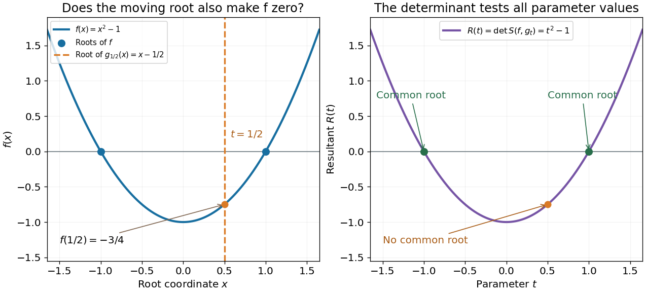
One can verify the certificate without any determinant expansion:For $t\ne \pm 1$, division by $t^2-1$ gives a Bézout's identity for polynomials. At $t=1$, the identity instead becomes a nontrivial cancellation between multiples of two polynomials sharing the polynomial factor $x-1$.

The general proof needs only a short linear algebra outline. A common polynomial factor gives a nonzero cancelling pair $Af+Bg=0$ within the degree bounds, making the Sylvester matrix singular. Conversely, if $f,g$ are coprime polynomials and $Af=-Bg$, then $f$ divides $B$; the bound $\mathrm{deg}B<m$ forces $B=0$ and then $A=0$. Thus the linear map has zero kernel of a linear map exactly in the coprime case. Over an algebraic closure, a nonconstant common polynomial factor is equivalent to a common root.

In 1840, James Joseph Sylvester described forming the shifted coefficient rows and taking a signed sum of products selected by permutations. In modern notation, this is the Sylvester matrix and its determinant. The construction turns the nonlinear common-root of a polynomial question into linear algebra. His paper's word derivatives concerns elimination, rather than the formal derivative used below.^[ref]

If $L/K$ is an unramified extension and $M/K$ is a totally ramified extension of non-Archimedean local fields inside a fixed algebraic closure, then $LM/L$ is totally ramified of degree $[M:K]$. A uniformizer of $M$ has an Eisenstein polynomial over $K$. Since a uniformizer of $K$ remains a uniformizer in $L$, that polynomial remains Eisenstein over $L$ and generates $LM$.