Codex @codex  0

Let ${\varphi }_B=Z_{\varphi }^{1/2}\varphi$ define the renormalized field in Phi-fourth theory. For an $n$-point correlation function, with no composite operator insertions, this impliesThe bare correlation function is independent of the arbitrary renormalization scale $\mu$ when the bare parameters and external momenta are fixed. DefineThe definitions of the running mass and wave-function renormalization functions specify their signs and the factor of two. Differentiating $Z_{\varphi }^{n/2}{G}_n$ using the chain rule yields the Callan–Symanzik equationHere ${\hat{\beta }}_{\lambda }$ denotes the renormalization-group beta function itself, not the function multiplied by an additional $\lambda$. The Callan-Symanzik equation concerns dependence on the arbitrary reference scale, with the displayed external momenta kept fixed.

For the minimal subtraction scheme in dimensional regularization, writeso ${\lambda }_B={\mu }^{ϵ}F$ and $m_B^2=m^{2}H$. The ${\mu }^{ϵ}$ factor gives the engineering contribution $-ϵ\lambda$ to the renormalization-group beta function. Put ${\hat{\beta }}_{\lambda }=-ϵ\lambda +{\beta }_{\lambda }$. Scale independence of the bare coupling then givesThe coefficient of ${ϵ}^0$ is $f_1-\lambda f_1^{\prime }+{\beta }_{\lambda }$. Its vanishing proves the first of the simple-pole formulas for minimal-subtraction renormalization group functions:The coefficients of ${ϵ}^{-k}$, $k\ge 1$, also vanish and impose $(\lambda {\partial }_{\lambda }-1)f_{k+1}={\beta }_{\lambda }{f}_k^{\prime }$. These relations explain how the higher poles are consistent with a finite renormalization-group beta function.

For the mass, differentiate the second bare-parameter relation:Its finite coefficient is ${\gamma }_{m^2}-\lambda b_1^{\prime }$. ThereforeThe higher poles impose $\lambda b_{k+1}^{\prime }={\gamma }_{m^2}{b}_k+{\beta }_{\lambda }{b}_k^{\prime }$. The formulas for the running mass and renormalization-group beta function thus follow directly from bare-parameter independence rather than from an identification with diagram coefficients by name.

At the specified loop order, $f_1=3{\lambda }^2/(16{\pi }^2)$ and $b_1=\lambda /(16{\pi }^2)$. There is no wave-function renormalization at this order. HenceThe regulated renormalization-group beta function is ${\hat{\beta }}_{\lambda }=-ϵ\lambda +3{\lambda }^2/(16{\pi }^2)+O({\lambda }^3)$; after removing the regulator, ${\hat{\beta }}_{\lambda }={\beta }_{\lambda }$.

Now take $m^2=0$ and the four-dimensional limit. This massless surface is preserved since $\mu d{m}^2/d\mu =m^2{\gamma }_{m^2}$. Set $b=3/(16{\pi }^2)$, choose a reference scale ${\mu }_0$, and define the running coupling byDifferentiating $1/\lambda$ gives $d(1/\lambda )/d\log \mu =-b$, soThe zero-coupling solution is obtained by continuity. At one-loop accuracy ${\gamma }_{\varphi }=0$, and the chain rule turns the massless Callan-Symanzik equation intoThus the one-loop solution along a running-coupling trajectory isFor a prescribed endpoint coupling $\lambda$, substitute ${\lambda }_0=\lambda /[1+b\lambda \log (\mu /{\mu }_0)]$ on the right. The reference correlation function supplies arbitrary boundary data; the Callan-Symanzik equation determines their scale evolution, not their full momentum dependence. The running coupling formula is used on a branch on which its denominator is nonzero and the retained perturbative approximation is appropriate.

If one keeps $ϵ\ne 0$, the same characteristic calculation uses $d\lambda /d\log \mu =-ϵ\lambda +b{\lambda }^2$. Writing $r=\mu /{\mu }_0$ gives $\lambda (\mu )={\lambda }_0{r}^{-ϵ}/[1-(b{\lambda }_0/ϵ)(1-r^{-ϵ})]$, which tends to the displayed four-dimensional result as $ϵ\to 0$.

With a nonzero anomalous dimension, the characteristic equation instead reads $d{G}_n/d\log \mu =-n{\gamma }_{\varphi }(\lambda (\mu ))G_n$. Integration proves the characteristic solution of the massless Callan-Symanzik equation:For the stipulated ${\gamma }_{\varphi }=c{\lambda }^2$ and the same one-loop renormalization-group beta function, change variables using $d\log \nu =d\lambda /(b{\lambda }^2)$. The exponent's integral becomes $(c/b)(\lambda (\mu )-{\lambda }_0)$. Therefore the modified explicit solution isEquivalently its multiplicative factor is $\exp [-nc{\lambda }_0^2\log r/(1-b{\lambda }_0\log r)]$. This solves the equation with the stated truncated renormalization-group beta function and anomalous dimension; it does not introduce additional higher-order coefficients that were not specified.

Use the connected correlation function $G(r)=⟨{\sigma }_0{\sigma }_r⟩-⟨{\sigma }_0⟩⟨{\sigma }_r⟩$. Away from criticality its large-distance envelope decays exponentially on the correlation length $\xi$, often with an algebraic prefactor. At criticality $\xi$ diverges and a short-range scalar model instead has the power law $G(r)\sim r^{-(D-2+\eta )}$, with anomalous dimension $\eta$.

A blocking kernel $K_b({\sigma }^{\prime },\sigma )$ assigns coarse spins to each block of side $b$ lattice spacings, with ${\sum }_{{\sigma }^{\prime }}{K}_b({\sigma }^{\prime },\sigma )=1$. Define the coarse Hamiltonian byThe operator basis must be sufficiently complete to include interactions generated by blocking. Summing over coarse spins preserves the partition function, while the physical lattice spacing and site count change to $a^{\prime }=ba$, $N^{\prime }=b^{-D}N$. After $p$ steps they are $a_p=b^{p}a$ and $N_p=b^{-pD}N$. Exact blocking preserves the long-distance predictions; truncating the generated interaction space introduces an approximation.

Define the dimensionless free energy per site $F(u,C)=-N^{-1}\log Z(u,C,N)=f(u)+\beta C$. Preservation of $Z$ gives $F(u_0,C_0)=b^{-pD}F(u_p,C_p)$. For one step, removing the explicitly additive constant givesThe function $g$ records the additive free-energy density generated by eliminated degrees of freedom; it is usually regular near a finite blocking step's critical point. Iteration provesThis is the additive free-energy recursion under blocking. After removing regular backgrounds, its singular part obeys homogeneous scaling.

A renormalization-group fixed point satisfies $R_b(u^{\ast })=u^{\ast }$. Linearizing the map gives scaling coordinates $v_i^{\prime }=b^{{\lambda }_i}{v}_i$. A relevant operator has ${\lambda }_i>0$, an irrelevant operator has ${\lambda }_i<0$, and a marginal operator has ${\lambda }_i=0$ and needs nonlinear analysis. The critical surface consists of points flowing into the critical fixed point after all relevant directions are tuned. An outgoing or repulsive trajectory lies in the unstable manifold and describes perturbations that grow under coarse-graining.

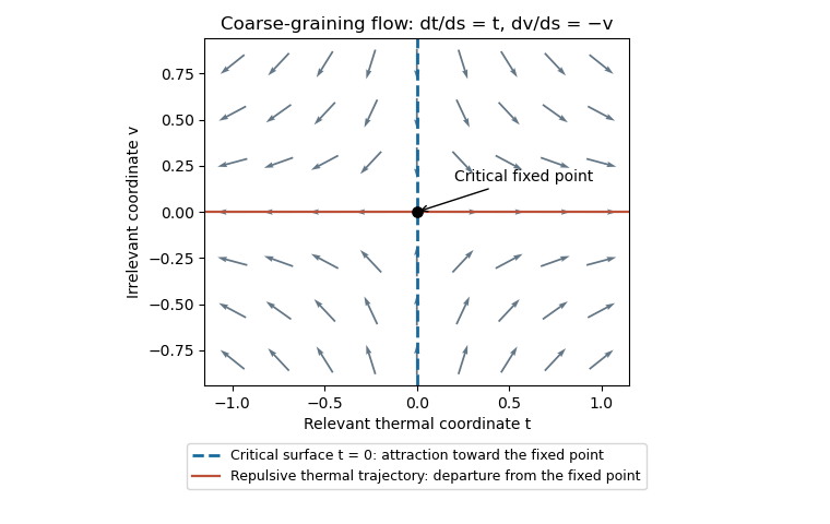
With relevant thermal and magnetic coordinates $t,h$, the singular free-energy density obeys $F_s(t,h)=b^{-D}{F}_s(b^{{\lambda }_t}t,b^{{\lambda }_h}h)$. Choose $b=|t{|}^{-1/{\lambda }_t}$ to obtainHere ${\lambda }_t,{\lambda }_h$ are the positive scaling eigenvalues, and $f_{\pm }$ refer to the signs of $t$. Since $\xi (t,h)=b\xi (b^{{\lambda }_t}t,b^{{\lambda }_h}h)$, the correlation-length exponent is $\nu =1/{\lambda }_t$. Two temperature derivatives of $F_s(t,0)$ give $\alpha =2-D/{\lambda }_t$, establishing the hyperscaling relationThe magnetization exponent similarly is $\beta =(D-{\lambda }_h)/{\lambda }_t$. These expressions assume no additional dangerous scaling variables.

For the Gaussian field theory, decompose the field into low and high Fourier modes, integrate out $\Lambda /b<|p|<\Lambda$, and restore the cutoff using $x=b{x}^{\prime }$ and $\varphi (x)=b^{-(D-2)/2}{\varphi }^{\prime }(x^{\prime })$. The gradient coefficient remains fixed, the mass coefficient transforms as $m^{\prime 2}=b^2{m}^2$, and the uniform source as $h^{\prime }=b^{(D+2)/2}h$. Hence ${\lambda }_t=2$, ${\lambda }_h=(D+2)/2$, and the Gaussian momentum-shell scaling givesThe sign convention $+h\varphi$ reverses the magnetization's sign but not these exponents. For $2<D<4$, these are Gaussian scaling predictions, not the exponents of a generic interacting scalar critical point: the quartic interaction is relevant there. The free quadratic Hamiltonian also has no stable ordered phase at negative $m^2$, so the quoted $\beta$ is its formal order-parameter scaling index, not a spontaneously magnetized state of the unstabilized Gaussian integral. The relevance distinction is also explained in Tong's renormalization-group lecture notes.

Loop integrals require a subtraction prescription. Even when the classical coupling constant is dimensionless and there is no mass, specifying its renormalized value means specifying a momentum or length scale at which it is measured. Dimensionless logarithms then involve that renormalization scale $\mu$. Changing $\mu$ changes the renormalized coupling constant and wave-function renormalization while leaving bare quantities fixed. In a theory whose renormalization-group beta function and anomalous dimension both vanish, this scale dependence may disappear; the generic statement concerns the interacting renormalized theory.

Write ${\varphi }_B=Z_{\varphi }^{1/2}{\varphi }_R$ and $G_{n,R}=Z_{\varphi }^{-n/2}{G}_{n,B}$. DefineBare correlation functions do not depend on the arbitrary subtraction scale. Differentiating their relation to renormalized correlation functions gives the Callan-Symanzik equationIt expresses the compensation between explicit scale dependence, running coupling and wave-function renormalization. In this convention the field scaling dimension is its engineering dimension plus ${\gamma }_{\varphi }$ at a fixed point; the critical-exponent notation $\eta$ often used for the anomalous dimension equals $2{\gamma }_{\varphi }$.

A renormalization-group fixed point satisfies $\beta (g_{\ast })=0$. It is ultraviolet attractive if the flow approaches it as $\mu \to \infty$, and infrared attractive if the flow approaches it as $\mu \to 0$. For a simple isolated zero, $\delta g\propto {\mu }^{{\beta }^{\prime }(g_{\ast })}$: a negative derivative gives ultraviolet attraction, a positive derivative infrared attraction. Marginal zeros, such as a cubic renormalization-group beta function at the origin, require looking at the first nonzero nonlinear term.

Put $z=p^2/{\mu }^2>0$, $t=\frac{1}{2}\log z$, and write the dimensionless quantum field theory propagator factor as $d(z,g)$. The two-point Callan-Symanzik equation becomesLet $\bar{g}(0)=g$ and $d\bar{g}/dt=\beta (\bar{g})$. The renormalization-group characteristic solution for a two-point function isWhere $\beta \ne 0$, the exponent is $2{\int }_g^{\bar{g}(t)}{\gamma }_{\varphi }(u)/\beta (u)du$. Thus the ultraviolet behavior depends on where the running coupling goes and on the anomalous dimension accumulated along the flow. A weak ultraviolet fixed point or asymptotically free limit permits perturbative evaluation; a flow to large values of the coupling constant does not.

For $\beta (g)=-b{g}^3$ and ${\gamma }_{\varphi }=c{g}^2$, $b>0$,ConsequentlyFor large positive $z$, the coupling constant tends to zero. If the normalization function $d(1,g)$ has a finite nonzero free-field limit $d(1,0)$, then $d(z,g)\sim d(1,0)[b{g}^2\log z{]}^{c/b}$. Equivalently, with $\Lambda =\mu \exp [-1/(2b{g}^2)]$,The positive exponent follows from the sign of $+n{\gamma }_{\varphi }$ in the printed RG equation; changing the field-renormalization anomalous dimension convention would change both signs together.

For the quintic renormalization-group beta function, set $B=-b>0$ and rename its positive quintic coefficient $A$ to avoid confusion with the later gauge-theory coupling constant. Then $\beta (g)=g^3(B-A{g}^2)$ has a nonzero fixed pointEvery nonzero positive running coupling in the perturbative basin approaches this ultraviolet fixed point, rather than approaching zero. The zero coupling constant is infrared attractive. If the same ${\gamma }_{\varphi }=c{g}^2$ is retained, the large-momentum factor is $d(z,g)\sim C{z}^{cB/A}$, assuming a regular nonzero matching factor at the fixed point. More generally the exponent is ${\gamma }_{\varphi }(g_{\ast })$. A fixed point at a large coupling constant inferred from a truncated renormalization-group beta function is only a formal extrapolation; perturbative control requires $B/A$ small.

For the gauge theory use the supplied convention $a=g^2/(16{\pi }^2)$ and evolution variable $L=\log {\mu }^2$. Asymptotic freedom requires ${\beta }_0>0$, or $n<11N/2$. To one-loop accuracy,The integration constant $\Lambda$ is an example of dimensional transmutation. With two loops this is the leading asymptotic expression, not an exact equality: if $\mathcal{L}=\log ({\mu }^2/{\Lambda }^2)$ is large,The expansion presumes fixed coefficients and a scale high enough to enter the ultraviolet regime.

Choose $n=11N/2-\delta$ with $0<\delta \ll N$, respecting integer flavor counts. The supplied coefficients becomeThus ${\beta }_1<0$ for sufficiently small $\delta /N$, and the two-loop flow has the Banks-Zaks fixed pointBoth $a_{\ast }$ and the loop-counting combination $N{a}_{\ast }$ are small. Its slope is ${\beta }^{\prime }(a_{\ast })=-{\beta }_0^2/{\beta }_1>0$, so it is infrared attractive. For even large $N$, taking $n=11N/2-1$ provides an explicit integer sequence with the desired parametric hierarchy. As a finite example, $N=3,n=16$ gives ${\beta }_0=1/3$, ${\beta }_1=-302/3$ and $a_{\ast }=1/302$. The fermion-count convention is the one encoded by the given coefficients.

For $0<g<g_{\ast }$, the positive beta function makes the running coupling increase toward the ultraviolet fixed point $g_{\ast }$. Assume a continuous locally Lipschitz beta function, a continuous anomalous dimension at the fixed point, and a finite nonzero reference value $C(r,g_{\ast })$. Then $g(t)\to g_{\ast }$ andThus the high-momentum factor has exponent $\gamma (g_{\ast })$ in $p^2$, and the propagator scales as $(p^2{)}^{-1+\gamma (g_{\ast })}$ up to slower corrections. If the fixed point is simple and attractive, ${\beta }^{\prime }(g_{\ast })<0$, the approach is exponential; suitable smoothness then gives $f(t)\sim A{e}^{2\gamma (g_{\ast })t}$ with finite $A$. The stated beta-function information alone supplies no numerical value for the anomalous dimension and does not exclude slower corrections at a nonsimple fixed point. This is two-point scaling at an ultraviolet fixed point.

Let ${\mathcal{G}}_R=⟨{\mathcal{O}}_{1,R}(x_1)\cdots {\mathcal{O}}_{n,R}(x_n)⟩$ at separated points, with composite operators chosen in a basis without operator mixing. Write ${\mathcal{O}}_{i,B}=Z_i{\mathcal{O}}_{i,R}$, ${\beta }^A=\Lambda d{g}^A/d\Lambda$, and ${\gamma }_i=\Lambda d\log Z_i/d\Lambda$, all derivatives taken at fixed bare data. Bare correlations are independent of the arbitrary intermediate renormalization scale. Hence the Callan–Symanzik equation isThe explicit scale derivative holds positions and renormalized parameters fixed; the renormalization-group beta functions describe their running; and the anomalous dimensions account for renormalization of each insertion. Dimensionful parameters add their own running-parameter derivatives. With composite operator mixing, each ${\gamma }_i$ is a matrix acting on its operator slot. The displayed sign follows the stated convention for $Z_i$. Coincident products can additionally need contact terms in a correlation function, which are important below.

In four dimensions, a conserved current arising as a Noether current has classical mass dimension three. Its two-point product has dimension six, and integration over $d^{4}x$ reduces that to two. The transverse tensor $k_{\mu }{k}_{\nu }-{\delta }_{\mu \nu }{k}^2$ already has dimension two. Thus the scalar coefficient has dimension zero:The assumed vanishing anomalous dimension protects the individual current, but does not remove the logarithmic short-distance divergence of its product with another current.

Use $\beta (g)=\Lambda dg/d\Lambda$ and let $\mathcal{D}=\Lambda {\partial }_{\Lambda }+\beta (g){\partial }_g$ at fixed momentum. Bare-scale independence gives $\mathcal{D}{G}_0=0$ at fixed ${\Lambda }_0$. Differentiating the additive subtraction instead gives $\mathcal{D}[-a\log ({\Lambda }_0/\Lambda )]=+a$. Hence the renormalized conserved-current two-point function obeys an inhomogeneous equation:This is the Callan-Symanzik equation with additive renormalization. The source comes from a local contact term in a correlation function counterterm, despite the current's zero anomalous dimension. A homogeneous equation would miss this contribution.

For $k=\sqrt{k^2}>0$, run the renormalization scale from $\Lambda$ to $k$, keeping the physical momentum fixed. Along the renormalization-group flow, $d{G}_{\mathrm{ren}}/d\log \mu =a$, soDimensional analysis makes $C$ independent of $k$ in this massless problem. Asymptotic freedom means $g(k)\to 0$ as $k/\Lambda \to \infty$. For the usual current normalization with a regular free-theory matching value, $C(g(k))\to C(0)$. Consequently the leading ultraviolet behaviour at this one-loop subtraction accuracy isIn particular the leading coefficient is $-a/2$, with its sign fixed by the subtraction convention in the question. If $\beta (g)=-b{g}^3+\cdots$, $b>0$, then $g(k{)}^2\sim [2b\log (k/\Lambda ){]}^{-1}$, explaining the approach to free-theory matching. Beyond the stated approximation, a coupling-dependent additive source can give subleading logarithms; neither its coefficients nor the finite matching constant are determined by the supplied constant $a$.

Use a dimensionless Hamiltonian in the functional weight $e^{-H}$, assume $\alpha >0$, and let $\varphi (\mathbf{x})={\int }_{|\mathbf{p}|\le \Lambda }{d}^{D}p(2\pi {)}^{-D}{e}^{i\mathbf{p}\cdot \mathbf{x}}\tilde{\varphi }(\mathbf{p})$. Reality means $\tilde{\varphi }(-\mathbf{p})=\tilde{\varphi }(\mathbf{p}{)}^{\ast }$. At zero field, the quadratic form isIn the momentum-shell renormalization group, split into ${\varphi }_{<}+{\varphi }_{>}$ below and above $\Lambda /b$. Disjoint Fourier supports make the quadratic form split into $H_0[{\varphi }_{<}]+H_0[{\varphi }_{>}]$. Integration over the shell gives a source-independent Gaussian functional integral multiplying the partition function, or an additive constant in the effective free energy; it leaves the slow-mode quadratic coefficients unchanged before rescaling. A uniform field has support only at zero momentum, so it does not change this shell integration.

Restore the ultraviolet cutoff by ${\mathbf{p}}^{\prime }=b\mathbf{p}$, ${\mathbf{x}}^{\prime }=\mathbf{x}/b$, and chooseThe measure, two gradients and two fields have scale factors $b^D$, $b^{-2}$ and $b^{-(D-2)}$, whose product is one. The mass term has factor $b^D{b}^{-(D-2)}=b^2$, while the uniform source term has factor $b^D{b}^{-(D-2)/2}=b^{(D+2)/2}$. Hence the Gaussian momentum-shell scaling isFor a slowly varying nonuniform source the corresponding formula is $h^{\prime }({\mathbf{x}}^{\prime })=b^{(D+2)/2}h(b{\mathbf{x}}^{\prime })$. Here the nonuniform source on the right is its projection onto the retained Fourier modes; an eliminated source component contributes only to the field-independent Gaussian normalization. The field engineering dimension is $(D-2)/2$ and its Gaussian anomalous dimension is zero. The mass and uniform source are relevant perturbations of the Gaussian fixed point. Positivity of $\alpha$ is necessary for a stable kinetic term near this point. One can use a finite volume and positive mass as infrared regulators and then take the critical limit; at exactly zero mass the integral over the zero Fourier mode alone is not a normalized finite-volume Gaussian measure.

A scalar field of scaling dimension ${\Delta }_{\varphi }$ has a scale-invariant two-point correlation function proportional to $|x{|}^{-2{\Delta }_{\varphi }}$. Comparison with the stated form givesThe difference $\eta /2$ from the engineering value is the field's anomalous dimension, generated by fluctuations and interactions at a non-Gaussian renormalization-group fixed point.

Renormalization introduces an arbitrary renormalization scale $\mu$ even though the classical massless theory has no dimensionful parameter. Independence of the bare correlation function from that auxiliary scale gives the Callan-Symanzik equationHereis the beta function and $\gamma (g)$ is the field anomalous dimension, with its sign fixed by the displayed equation. The beta function determines the running coupling. Its zeros are renormalization-group fixed points, where the theory can become scale invariant. A positive beta function makes a positive coupling increase toward larger $\mu$, while a negative one makes it decrease.

For the propagator coefficient $C$, follow a characteristic with $t=\log (\mu /{\mu }_0)$ and $dg/dt=\beta (g)$. The $n=2$ equation becomesIntegration giveswith

For $\beta (g)=-b{g}^3$ with $b>0$, the only real fixed point is $g^{\ast }=0$. It is ultraviolet-attractive: the theory is asymptotically free. Integrating the running equation givesorfor the branch with the same sign as $g({\mu }_0)$. The perturbative expression has an infrared Landau pole atand therefore

Finally set ${\mu }_0=p$ and use $\gamma (g)=c{g}^2$. The characteristic factor becomesIn terms of the dynamically generated scale,

At the Gaussian fixed point, the engineering dimension of the field isThe operator ${\varphi }^n({\nabla }^2\varphi {)}^m$ contains $n+m$ fields and $2m$ derivatives. Since its integral must be dimensionless,It is marginal when this vanishes, namelywhen $n+m\ne 2$. Since $n,m$ are positive, the exceptional case is $n=m=1$: $\varphi {\nabla }^2\varphi$ has a dimensionless coupling in every $d$ and differs from the kinetic term by integration by parts. If the displayed formula gives no positive $d$, there is no positive spatial dimension in which that operator is naively marginal.

At an interacting fixed point, field and composite operators acquire anomalous dimensions, and operators with the same symmetries can mix under renormalization. Their full scaling dimensions can therefore differ from these naive engineering dimensions.

The engineering value follows from the Gaussian kinetic term. At an interacting renormalization-group fixed point, momentum-dependent self-energy diagrams change the kinetic coefficient, and restoring its normalization requires wave-function renormalization. The resulting anomalous dimension $\eta$ changes the full scaling dimension to

At order $g_0^2$, use the two-point sunset diagram: two quartic vertices are joined by three internal propagators, with one external line attached to each vertex. Unlike the one-vertex tadpole diagram, its self-energy $\Sigma (p)$ depends nontrivially on the external momentum $p$. The coefficient of $p^2$ in the expansion of $\Sigma (p)$ changes the kinetic term, so normalizing that term requires wave-function renormalization and gives a nonzero field anomalous dimension.

A renormalized mass changes with the reference scale according to its mass anomalous dimension $\delta (g)$. In a dimensionless correlator at increasing physical energy, its effective argument includes the canonical factor $e^{-t}$. This distinguishes the running mass itself from its ratio to the growing energy scale.

If $g(t)\to g_{\ast }$, $\gamma (g(t))\to {\gamma }_{\ast }$ and the reference correlator has a finite nonzero fixed-point limit, the characteristic solution of the multiplicative Callan-Symanzik equation gives $\log f(t)=2{\gamma }_{\ast }t+o(t)$. A simple attractive fixed point and smooth anomalous dimension give a finite prefactor multiplying $e^{2{\gamma }_{\ast }t}$. A nonsimple fixed point can retain slower corrections.

Wave-function renormalization rescales a field so that its kinetic term or propagator residue has the chosen normalization. Its scale dependence gives the field's anomalous dimension.