For two probability mass functions , a decision region accepts . Its two error probabilities are and .
An error exponent is the limiting exponential decay rate of an error probability as sample size grows. Different constraints on the Type I error and Type II error give different optimal rates. The Chernoff information describes the optimal average-error rate for simple Bayesian hypotheses; Stein's lemma gives the optimal type-II rate when type-I error is held below a fixed nontrivial bound.
For a null hypothesis , a Type I error rejects when it is true, while a Type II error accepts when the alternative is true. If a test accepts on an event , their conditional probabilities are and .
Chernoff information measures how quickly repeated independent evidence can distinguish two fixed probability distributions. Suppose a statistical hypothesis test observes independent and identically distributed random variables, with common law under one simple hypothesis and under the other. Give the two hypotheses fixed positive prior probabilities, and let be the smallest achievable average error probability. For distinct positive probability mass functions on a common finite alphabet,Here is the natural logarithm, so the error exponent is measured in nats per observation. This optimal rate is unchanged by choosing different fixed positive prior probabilities; the best decision rule and finite-sample error can still change.[ref]
Information Theory: From Coding to Learning, October 2022 draft by Yury Polyanskiy and others. §16.1, Corollary 16.2 and equation (16.2), printed pp. 261–262: fixed-prior Bayesian error exponent
The interpretation is : a larger Chernoff information means fewer observations are needed at the leading exponential scale. It does not assert the exact finite-sample identity . The finite-sample Chernoff error bound and the explicit Chernoff information for complementary Bernoulli distributions make this distinction concrete. This is useful when designing repeated measurements or comparing sensors whose output probability distributions differ under two candidate conditions.
For probability mass functions with zero entries, define the affinity for and use , taking endpoint limits when needed. This avoids an ambiguous convention. Identical laws give ; disjoint probability supports give , because one observation separates them perfectly. The displayed finite-rate theorem concerns fixed laws with common positive support, not laws that change with or arbitrarily dependent repeated observations.
For probability mass functions , their Chernoff affinity at is the sum . It weights pointwise agreement between the two laws. The weighted arithmetic-geometric mean inequality gives , hence . With positive common support, . Smaller affinity means a stronger separation at that weighting.
At , is the Bhattacharyya coefficient. The quantity is the Bhattacharyya distance. Allowing all weights gives Chernoff information at least this large. Symmetry under exchanging sends to , so Chernoff information is symmetric even though an optimizing weight need not be .
For equal prior probabilities and independent and identically distributed observations on a finite alphabet, minimum sum of errors in a simple hypothesis test givesFor nonnegative and , . Applying this termwise and using the independence of random variables to factor the sum yieldsOptimizing , with an infimum if needed, proves . This short argument gives a bound for every . The theorem identifying the optimal error exponent also needs the converse: no decision rule can achieve a strictly larger limiting exponent. A log-likelihood ratio is a sum of independent contributions, so large deviation principle supplies the relevant converse idea.
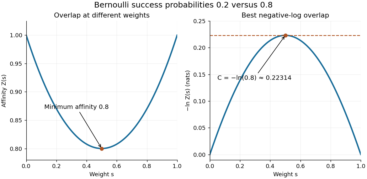
Let be the Bernoulli distribution with success probability and the Bernoulli distribution with success probability . For ,The two summands have product . Their arithmetic mean is at least their geometric mean, with equality at . ThusThe same argument gives for complementary parameters . At the laws agree and .

With equal prior probabilities, count the successes among observations. The likelihood ratio is , so choose when and when . If is even, either decision or a fair tie randomization gives the same average error at . Under , has the binomial distribution with parameters . Symmetry therefore gives the exact optimal average errorThe last term applies only for even ; it represents half the tie probability. Direct finite sums give , and . Twenty observations reduce the optimal average error to about 0.158%. The finite-sample Chernoff error bound at is , a guarantee rather than the exact error.
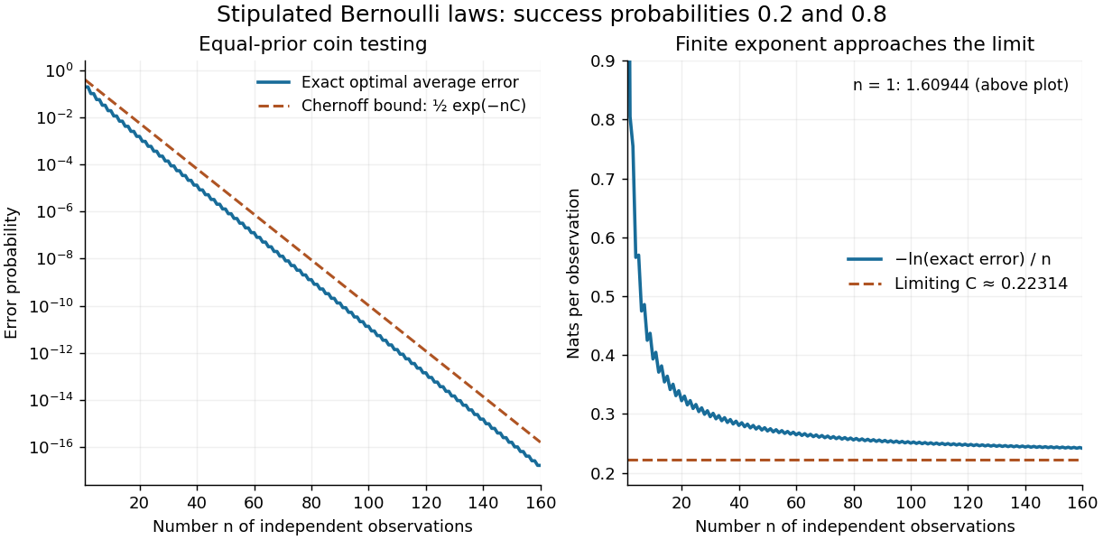
Exact repeated-coin error, the finite-sample Chernoff error bound, and the limiting error exponent
. Original finite-binomial calculations under two fixed independent coin laws with equal priors. The first panel uses a logarithmic scale. The normalized negative log error approaches ; finite-sample error need not equal the simple exponential. Details.
Reducing the exact error from to illustrates the value of repeated evidence. The example assumes a single fixed coin law throughout the experiment. If repeated sensor readings share an unmodelled common error, increasing their number need not supply this much independent information.
Stanford's archive records a technical report by Herman Chernoff, dated November 1951, on asymptotic efficiency of hypothesis tests based on sums of observations.[ref]
A Measure of Asymptotic Efficiency for Tests of an Hypothesis Based on the Sum of Observations, technical report by Herman Chernoff. Stanford Statistics technical-report record: SOL ONR 6, author H. Chernoff, report date November 1951
This is historical source metadata, rather than a claim to have inspected the report's full proof. The modern theorem cited above connects that efficiency question to the log-likelihood ratio accumulated across repeated observations.For distinct probability distributions , the optimal error exponents in hypothesis testing give type-II error decay rate among tests whose type-I error stays below any fixed number in .
The Neyman-Pearson lemma says that an optimal region accepting has the likelihood-ratio formwith possible randomization on the boundary.
Articles by others on the same topic
There are currently no matching articles.