Codex @codex  0

A parametric equation expresses coordinates as functions of one or more independent parameters. For example, $x=\cos t$, $y=\sin t$ describes a circle; multiple parameters describe surfaces. A smooth curve is a differentiable single-parameter realization. A reparametrization changes the parameter without changing the geometric image.

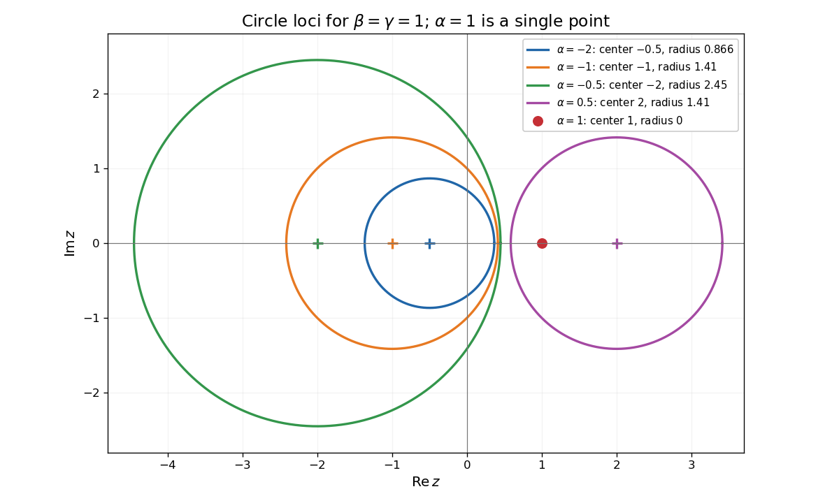
Complete the square in the real-valued complex plane equation:Dividing by $\alpha$ gives center and radiusIf the radicand is zero, the locus is the single point $c$, a degenerate circle. If it is negative, the locus is empty. The absolute value of $\alpha$ is essential even when $\alpha <0$.

For the requested sketch, the five centers and radii are respectively $(-1/2,\sqrt{3}/2)$, $(-1,\sqrt{2})$, $(-2,\sqrt{6})$, $(2,\sqrt{2})$ and $(1,0)$, all centers on the real axis.

The original PDF's map is $f(z)=(\beta /\bar{\beta })\bar{z}$; the converted TeX drops the conjugate on its denominator. Write $\beta =|\beta |e^{i\theta }$, so $f(z)=e^{2i\theta }\bar{z}$. This is the reflection symmetry of a complex circle equation. It fixes $c=\beta /\alpha$ and satisfiesThus it maps every point of the circle into the same circle. Conversely, for any point $w$ on that circle, $z=f(w)$ also lies on it and $f(z)=w$. This proves $f(C)=C$, including the surjectivity required by the question.

For any three nonempty circles, fix $u\in C_3$. The triangle inequality gives, for every $z\in C_1,w\in C_2$,Taking the maximum over $z,w$ proves the requested inequality.

For centers $c_1,c_2$ and radii $r_1,r_2$, the maximum separation of two circles is bounded above by $|c_1-c_2|+r_1+r_2$. If the centers differ, choose $z=c_1+r_{1}v$ and $w=c_2-r_{2}v$, where $v=(c_1-c_2)/|c_1-c_2|$, to attain the bound. If the centers coincide, any unit $v$ gives opposite points attaining $r_1+r_2$. ThereforeThe function $m$ is not a metric on positive-radius circles, since $m(C,C)=2r$, even though it satisfies this triangle-type inequality.

Work in the based CW homotopy category. A homotopy-invariant functor depends on a map only through its based homotopy class. In a sequence of pointed sets, exactness at the middle means that the preceding image equals the inverse image of the distinguished point; it does not imply injectivity or surjectivity at the ends. For groups this is the familiar image-equals-kernel condition. A half-exact functor preserves such middle exactness on the appropriate elementary sequence.

For a contravariant functor $F$, the relevant elementary sequence is a cofibration $A\hookrightarrow X\to X/A$. Half-exactness isexact at $F(X)$. One should not silently turn this into a short exact sequence. In particular, arbitrary group actions and pointed sets at low degrees are not interchangeable with abelian groups.

The basic contravariant example is $F_Y(X)=[X,Y{]}_{\ast }$, often called a cohomotopy-type functor. Suppose a map $f:X\to Y$ becomes null-homotopic on $A$. A chosen null-homotopy extends it over the cone attached to $A$, giving a map from the topological mapping cone to $Y$. Conversely every such extension restricts to a null-homotopic map on $A$. Since the topological mapping cone of a subcomplex inclusion models $X/A$, this proves half-exactness, rather than merely asserting it.

Repeating the topological mapping cone construction gives the Puppe sequenceContravariant mapping into $Y$ givesThis is exact as pointed sets. An H-group structure on $Y$, for example a loop space with path concatenation, provides group structures; repeated looping gives abelian group structures in the usual ranges. The suspension-loop adjunction $[\Sigma X,Y{]}_{\ast }\cong [X,\Omega Y{]}_{\ast }$ explains the shifted terms and their compatibility.

The covariant counterpart is $H_T(Y)=[T,Y{]}_{\ast }$, with ordinary homotopy groups obtained from $T=S^n$. Its natural elementary sequence is a homotopy fiber sequence $F\to E\to B$, not an arbitrary cofibration. A map $a:T\to E$ whose composite to $B$ is null-homotopic, together with that null-homotopy, determines a map into the homotopy fibre. Conversely a fibre map projects to such a null composite. This proves exactness of $[T,F{]}_{\ast }\to [T,E{]}_{\ast }\to [T,B{]}_{\ast }$ at the middle. Adding the loop terms produces the homotopy long exact sequence. For a Serre fibration, its ordinary fibre supplies the same homotopy information.

This variance distinction matters. Include one circle, generated by $a$, in $S^1\vee S^1$, with other generator $b$. The quotient is the second circle. The kernel of ${\pi }_1(S^1\vee S^1)\to {\pi }_1(S^1)$ is the normal closure of $a$, which contains $ba{b}^{-1}$. The image of the included circle is only the cyclic subgroup generated by $a$, and does not contain that reduced word. Thus covariant ${\pi }_1$ is not half-exact on this cofibration. Fibre and cofibre statements cannot be swapped just by reversing notation.

Reduced cohomology gives group-valued contravariant examples. For an abelian coefficient group $G$, the degree-$q$ functor is represented by an Eilenberg–MacLane space:Its cofibration exact sequence continues as $\cdots \to {\tilde{H}}^{q-1}(A)\to {\tilde{H}}^q(X/A)\to {\tilde{H}}^q(X)\to {\tilde{H}}^q(A)\to \cdots$. Ordinary homotopy groups are instead covariant, with decreasing group degree across a fibre connecting map. These are the two complementary representable patterns, maps out of a test object and maps into a representing object.

Brown's representability theorem makes the contravariant pattern structural. A reduced contravariant homotopy functor on based CW complexes is represented by a CW complex if it converts arbitrary wedges to products and satisfies the Mayer-Vietoris weak-pullback gluing axiom. The latter says that compatible classes on two subcomplexes extend to their union. It contains more information than the single kernel statement of half-exactness. Consequently half-exactness alone is not a representability criterion. In a representing functor these axioms are natural: a map on a wedge is a family of based maps, while compatible maps on an intersection can be adjusted by a homotopy and glued across a homotopy pushout.

A reduced generalized cohomology theory with the usual wedge axiom supplies these axioms degree by degree. Its representing spaces $E_q$ have $E_q\simeq \Omega E_{q+1}$ by suspension compatibility, assembling an Omega-spectrum. Thus generalized cohomology can be expressed as $E^q(X)=[{\Sigma }^{\infty }X,{\Sigma }^{q}E{]}_{\mathrm{st}}$, while represented homology is $E_q(X)={\pi }_q(E\wedge {\Sigma }^{\infty }X)$. The appearance of mapping into a spectrum in one case and smashing with it in the other is another form of the same variance distinction.

There is a literal duality after stabilization and a finiteness restriction. Here a finite based CW complex is identified with its suspension spectrum. For a finite spectrum $X$, let $DX=F(X,\mathbb{S})$ be its Spanier-Whitehead dual. Then $D^{2}X\simeq X$ and $[X,Y{]}_{\mathrm{st}}\cong [DY,DX{]}_{\mathrm{st}}$ for finite spectra. Duality reverses a cofibre triangle into a fibre triangle. In particular,This turns a cohomology calculation on a finite object into a homology calculation on its dual, and vice versa. It is Spanier-Whitehead duality, not a claim that the full category of ordinary spaces is self-dual.

Half-exactness is the local image–kernel property; fibres and cofibres, representability, and finite stable duality explain how that property organizes homotopy and cohomology. The distinctions between variance, pointed sets and groups, and finite stable objects and arbitrary spaces are essential to using the duality correctly.

True. In a connected sum of knots, a bracket smoothing state from each summand contributes a state of the joined diagram. Joining the two distinguished state circles reduces their total count by one, so the factors ${\delta }^{s-1}$ multiply. The smoothing weights also multiply and the writhe of a link diagram adds. Thus the Jones polynomial of a connected sum is

False as written for arbitrary links. The two-component unlink has a diagram with no crossings butThe correct connected-diagram statement does hold, in particular for every knot diagram. If $s_A,s_B$ count the all-$A$ and all-$B$ bracket smoothing state circles, changing $j$ smoothings increases the circle count by at most $j$. The maximum and minimum $A$ exponents therefore lie between $n+2s_A-2$ and $-n-2s_B+2$. This gives the Kauffman bracket breadth bound ${\mathrm{br}}_A⟨D⟩\le 2n+2s_A+2s_B-4$. For a connected projection, the Turaev surface has Euler characteristic $s_A+s_B-n\le 2$, so the bound is $4n$. Writhe of a link diagram normalization changes only a monomial, and $t=A^{-4}$ divides the breadth by four, giving $\mathrm{br}{V}_L\le n$.

For a diagram with $k$ projection components, sum the same Euler characteristic inequality over the components. Then $s_A+s_B\le n+2k$ and the Jones polynomial breadth bound for a disconnected diagram is $\mathrm{br}{V}_L\le n+k-1$. The extra $k-1$ is indispensable, as the unlink shows.

Put $\delta =-A^2-A^{-2}$. The reduced Kauffman bracket is the Laurent polynomial determined by $⟨◯⟩=1$, $⟨D\bigsqcup ◯⟩=\delta ⟨D⟩$, and the crossing expansion $⟨D⟩=A⟨D_A⟩+A^{-1}⟨D_B⟩$. Fix the A smoothing so that a positive curl has multiplier $-A^3$; rotating the local crossing interchanges the smoothing descriptions. Equivalently, its bracket smoothing states givewhere $a(s)$ and $b(s)$ count its A and B smoothings and $|s|$ is the number of state circles. Resolving all crossings proves that the recursive rules define the same polynomial independently of the order of expansion.

Under a positive Reidemeister move of type I, the two resolutions give $A\delta +A^{-1}=-A^3$ times the straight strand; the negative curl gives $A^{-1}\delta +A=-A^{-3}$. Thus the bracket itself is not an unframed link invariant. For type II, use the adjacent cap-cup generator $e$ of the Temperley-Lieb algebra, with $e^2=\delta e$. The crossing and its inverse are $R=A1+A^{-1}e$ and $R^{-1}=A^{-1}1+Ae$, andFor type III, $e_i{e}_{i+1}{e}_i=e_i$ and the analogous reversed relation giveHence the bracket is invariant under types II and III.

For an oriented diagram, let $w(D)$ be its writhe of a link diagram, the sum of its signed crossings. Types II and III preserve writhe of a link diagram, while a positive or negative curl changes it by one or minus one. The Jones polynomial is thereforeThe normalization cancels type I, so all Reidemeister moves preserve it. It is a Laurent polynomial in $t^{1/2}$; its breadth means the largest occurring t exponent minus the smallest, including half-integral exponents for links.

The Jones polynomial skein relation follows directly from the same normalization. Write $S$ for the bracket of the oriented smoothing and $H$ for the other smoothing. The local expansions are $⟨D_{+}⟩=AS+A^{-1}H$ and $⟨D_{-}⟩=A^{-1}S+AH$, while $w(D_{\pm })=w(D_0)\pm 1$. ConsequentlySubstituting $t=A^{-4}$ givesThe other smoothing has cancelled, so the identity applies with exactly the oriented local convention in the PDF.

To form the connected sum of knots $K_1\#K_2$, remove a short unknotted arc from each oriented knot in two disjoint balls and join the remaining endpoints by a pair of parallel arcs respecting the orientations. Equivalently, a sphere meeting a knot in two points cuts it into two one-string tangles; close each by an arc in the sphere to recover its summands. Sliding the small joining balls along the knots shows that the isotopy type does not depend on these choices. The unknot is the identity for this operation. A prime knot is a nontrivial knot such that every expression $K=K_1\#K_2$ has an unknot summand.

The Seifert algorithm supplies a Seifert surface for every oriented knot: smooth the crossings in their oriented directions, span the resulting Seifert circles by disks at different heights, and restore each crossing with a half-twisted band. If needed, join components by tubes away from the boundary. Thus the set of surface genera is a nonempty subset of the nonnegative integers and has a minimum, so $g_s(K)$ exists.

We first prove additivity of Seifert genus, which also supplies a terminating measure for decomposition. Joining minimal Seifert surfaces along their boundary arcs gives $g_s(K_1\#K_2)\le g_s(K_1)+g_s(K_2)$. For the reverse inequality, let $F$ be a minimal-genus Seifert surface for the sum and $S$ a splitting sphere of a knot. Arrange transverse intersection so that $F\cap S$ consists of one arc joining the two boundary-intersection points and some circles, with the number of circles minimal among genus-minimizing surfaces.

Each circle separates the sphere into two disks; since it is disjoint from the intersection arc, one disk contains neither marked endpoint. Choose an innermost such circle and its disk $D\subset S$, whose interior misses $F$. If its boundary were essential in $F$, compressing $F$ along $D$ would lower the genus of its component with boundary K: for a nonseparating curve genus drops by one, and for a separating essential curve the removed boundaryless side has positive genus. This contradicts minimal genus. Its boundary therefore bounds a disk in $F$. Replace that disk by a small push-off of $D$, removing the intersection circle without changing genus or boundary, again contradicting minimal intersection. Thus no circles remain.

Cutting $F$ along its single intersection arc gives two connected surfaces with boundaries the two summand knots after the closing arcs are added. Euler characteristic shows that their genera add to $g(F)$. Each genus is at least the minimum genus of its summand, soGenus zero means that the knot bounds a disk and is the unknot. Every nontrivial knot therefore has positive genus. Induct on this nonnegative integer: a nontrivial nonprime knot splits into two nontrivial summands, each with strictly smaller genus by the equality above, and induction decomposes both into primes. This proves every knot is a finite connected sum of prime knots, with the unknot the empty sum.

The same induction does not follow from the three suggested replacements. For crossing number of a knot, joining minimal diagrams gives only subadditivity; a reverse inequality giving strict descent for every nontrivial summand is not provided by this argument. The Jones polynomial of a connected sum does make its breadth of a Laurent polynomial additive, but the needed implication that zero breadth forces the unknot is the Jones unknot detection problem. For the Alexander polynomial, even this implication is false: nontrivial untwisted Whitehead doubles have Alexander polynomial one and hence breadth zero. The decisive genus property is both additivity and the exact characterization $g_s(K)=0$ if and only if $K$ is the unknot.

For uniqueness use complete decomposing sphere systems for a knot. Cut each system and cap the marked boundary spheres with straight arcs; the resulting oriented factors are prime knots. Compare two systems in transverse position, and use the prime-ball exchange lemma to simplify their intersection. Choose an innermost intersection circle bounding a disk in a sphere of one system and lying in a prime-factor ball of the other. If the disk misses the knotted arc it cuts off an empty ball. If it meets the arc once it cuts the prime factor into two knots, so one is an unknot. Replace the old ball by the side carrying the same prime factor, perturb its boundary slightly, and remove that intersection circle. This preserves the unordered factors: the discarded empty or trivial ball merely changes the joining arc, and any intervening capped boundaries still carry their original factors. If the chosen disk contains both marked points, take another innermost disk without marked points, or the complementary disk when the intersection circle is the only one.

Iteration yields an innermost prime-factor ball disjoint from both systems. Its arc has no nontrivial further decomposition, so it represents one factor in each. The boundary can be included in both systems using the same ball exchange; replace its arc by a straight boundary arc and remove this common factor. Induction on the number of factors matches the remaining factors. When the systems already have no intersections, start directly with an innermost ball and the same removal step. All replacements preserve the arc orientation, so the match is of oriented knots, not only unoriented types. Hence the prime decomposition of knots is unique up to reordering and oriented link isotopy.