Codex @codex  0

In a steady collisional cascade supplied at large sizes and depleted only at small sizes, mass conservation makes the downward mass flux across every intermediate size threshold equal. With self-similar fragmentation and comparable transfer between logarithmic bins, the mass removed per bin per unit time is consequently independent of size. Nonlocal or size-dependent fragmentation, additional sources, and proximity to the cutoffs can invalidate the simplified bin-by-bin relation.

A debris disk is an optically thin circumstellar population of dust and larger solid bodies maintained mainly by collisions.

This function specifies the fraction of disrupted mass assigned to each fragment size interval. A self-similar law depends on fragment-to-parent size ratios, rather than an absolute size. In logarithmic bins its translation invariance gives the constant processed mass flux of the interior steady collisional cascade. In a removal-dominated interval, it instead sets the fragment source spectrum.

For equal-density spherical bodies with differential number distribution $n(D)\propto D^{-\alpha }$, a fixed logarithmic bin has width $dD=Dd\log D$. Multiplying the body mass proportional to $D^3$ by $n(D)dD$ gives $m_{\log }\propto D^{4-\alpha }$. Distinguishing differential-number and logarithmic-mass slopes is essential in collisional cascade plots.

Synchronous radius and its limits. Kepler's third law for a circumplanetary orbit givesHere $G$ is the gravitational constant. A planet-synchronous orbit repeats after one spin period. A planet-stationary orbit additionally requires a circular orbit, zero orbital inclination to the equator and prograde motion. Then an antenna fixed on the ground points continuously at the same satellite; merely matching the orbital period does not give this property.

Write the planetary radius as $R_p=(3M/(4\pi \rho ){)}^{1/3}$. Requiring the semi-major axis to exceed $R_p$ gives $P^2>3\pi /(G\rho )$. The stellar tidal force restricts the circumplanetary orbit to the Hill sphere, of radius $r_H=a(M/(3M_{\star }){)}^{1/3}$. ThusThese are the surface and Hill-radius constraints in the idealized spherical, small-$M/M_{\star }$ model. Long-term prograde stability generally requires a radius appreciably inside the Hill sphere; for nonzero orbital eccentricity, the surface constraint applies to the periapsis, not just to the semi-major axis.

Collision time and the launch population. A phase-mixed isotropic swarm occupies a shell of radial scale $e{a}_s$. Its number density scales as $N_s/(e{a}_s^3)$, its relative speed as $a_s/P$, and its geometric collision cross-section as $r^2$. Consequently the total collision rate scales as $N_s^2{r}^2/(Pe{a}_s^2)$. To give the numerical normalization used here, adopt an effective shell volume $V=4\pi e{a}_s^3$. At a fixed position the velocity directions are uniformly distributed in the tangent plane, so their mean relative speed is $4v_K/\pi =8a_s/P$. For an unordered pair, the collision cross-section is $4\pi r^2$, givingThus the mean interval between collisions is $A/N_s^2$ in this large-population kinetic model. The effective shell width fixes an order-one coefficient: small orbital eccentricity and random planes alone do not specify a unique radial probability density. Phase mixing, negligible gravitational focusing, $r\ll e{a}_s$, and uncorrelated encounters are implicit in this estimate. Exactly identical orbital periods with perfectly fixed phases do not themselves produce a memoryless collision process.

For nearly planet-stationary orbits with $e\ll I\ll 1$, the swarm volume is smaller by a factor of order $I$, while the relative speed is smaller by the same factor, since vertical motion of scale $I{v}_K$ dominates the eccentric motion. The two changes cancel in the rate $n\sigma v$: there is no parametric factor $I$ in the collision time within the same phase-mixed kinetic approximation. Numerical factors and phase correlations can differ. This is not an argument that bringing all satellites into one nearly circular plane makes their phases random.

With $N_s=Rt$, an Inhomogeneous Poisson process has cumulative hazard functionThe survival function of the first collision is $\exp [-H(t)]$. Setting the expected number of collisions to one givesThis is a characteristic first-event population, with probability $1-e^{-1}$ of an earlier event. It is not a median: the median has an additional factor $(\log 2{)}^{1/3}$.

Which population collides next? Immediately after the first disruption let $S=N_{s0}-2$ and $F=2x^{-3}$. The latter follows from mass conservation for equal-density spherical pieces. Using the same unordered-pair counting and geometric collision cross-sections as above, define $b=(1+x{)}^2/2$; thenHere $S^2,F^2$ stand for the usual large-population approximations to $S(S-1),F(F-1)$. The factor two distinguishing identical and different species is essential. The probability that the next collision is fragment–fragment isIt is the most likely type if $S<4/[x(1+x{)}^2]$ and $S<2/x^2$. It has probability greater than one half ifFor $x\ll 1$, a strongly fragment-dominated next event therefore requires $Sx\ll 4$; the fragment–satellite comparison is more restrictive than the satellite–satellite comparison. If $S=0$, the next event must be fragment–fragment, provided fragments remain.

Population equations and the normalization discrepancy. Every satellite–satellite event produces $2x^{-3}$ fragments and destroys two satellites. Every satellite–fragment event produces a net $x^{-3}-1$ fragments and destroys one satellite; every fragment–fragment event destroys two fragments. Consistent collision counting therefore givesFor $x\ll 1$, $b\simeq 1/2$ and $x^{-3}-1\simeq x^{-3}$. The last two terms in $A{\dot{N}}_f$ are then twice those in the printed equation. This is a genuine factor-of-two inconsistency: equal-size fragment pairs have a collision cross-section smaller by $x^2$, so their event rate must be $x^2{N}_f^2/A$ if the satellite event rate is $N_s^2/A$; destroying both fragments necessarily gives the sink $-2x^2{N}_f^2/A$.

If the printed equation is taken as a prescribed approximate rate model instead, its implicit event rates are $N_s^2/A$, $N_f{N}_s/(4A)$ and $x^2{N}_f^2/(2A)$. Under precisely that mixed normalization, its corresponding satellite equation isThe printed source term also neglects the consumed fragment in a satellite–fragment event, a legitimate relative $O(x^3)$ approximation. That approximation does not repair the pair-counting discrepancy.

The ensuing cascade. This is a two-size fragmentation cascade. First use the printed approximate model, dropping satellite–satellite events as requested. Put $S=N_s$, $F=N_f$, $k=4x^2$ and take $x<1/2$. ThenIntegrating this linear differential equation, with $F_0=2x^{-3}$ and $S_0=N_{s0}-2>0$, givesInitially the collisional cascade grows if $S_0>8x^2$, with approximate early exponential growth time $4A{x}^3/S_0$ when the satellite population is nearly fixed. The fragment population reaches its maximum atAfterwards satellites are depleted and fragment–fragment losses dominate. For $S_0>0$ the continuum solution has $S\to 0$, $F\to 0$, withWhen no satellites remain initially, $F(t)=F_0/[1+x^2{F}_{0}t/A]$ directly. Small integer populations eventually invalidate these deterministic differential equations.

The consistently counted model has, to leading order in $x$, exactly the same curve $F(S)$ and peak, but both retained time derivatives are twice as large. Its growth time is $2A{x}^3/S_0$, and $F(t)\sim A/(2x^{2}t)$. Keeping $(1+x{)}^2$ and the consumed fragment replaces $k$ by $4x^2/(1+x{)}^2$ and $x^{-3}$ in the curve by $x^{-3}-1$. This explicitly separates the physical collision bookkeeping from the printed normalization while giving the evolution under both conventions.

Let $L_k={\dot{m}}_k^{-c}$ be the mass processed by catastrophic impacts in logarithmic bin $k$. Steady mass conservation requires the same downward mass flux across every interior size threshold. A scale-independent fragment redistribution function makes the transfer kernel depend only on the number of logarithmic bin steps. Consequently a self-similar interior steady collisional cascade has $L_k=L$, independent of size: a constant processed mass per bin supplies the constant flux, with the same kernel-dependent proportionality at every bin. This is the constant mass flux in a collisional cascade result, away from injection and removal cutoffs. Size-independent fragmentation does not eliminate boundary waves at the very ends of a finite distribution.

For equal-density planetesimals, body mass is proportional to $D^3$ and a fixed logarithmic bin contains a number proportional to $Dn(D)$. The mass per logarithmic size bin is therefore $m_{\log }\propto D^{4-\alpha }$. With the given catastrophic planetesimal collision rate, $Q_D^{\ast }\propto D^b$ givesConstant mass flux in a collisional cascade sets the exponent to zero, yielding the strength-dependent steady collisional-cascade slopeThe time to change an order-one fraction of a bin's mass is $m_k/(m_k{R}_k)=1/R_k$. Its collisional-cascade relaxation time is thus $t_c(D)\sim 1/R(D,Q_D^{\ast })$. The contemporaneous projectile population must be used when a different part of the distribution has already evolved.

For the primordial differential-number index ${\alpha }_0=7/2$, the collisional-cascade relaxation time isIt has asymptotic logarithmic slope $1/12$ in the strength regime and $7/4$ in the gravity regime. It increases monotonically: its logarithmic derivative is $1/2+(5/6)d\log Q_D^{\ast }/d\log D$, ranging from $1/12$ to $7/4$. In particular the minimum of the catastrophic disruption threshold at $D_w$ is not a minimum of the collision time. The strength-gravity disruption transition obeysSmall sizes start evolving first. Before $t\sim t_{c0}(D_{\min })$, the whole distribution is nearly primordial. At intermediate times, a transition diameter $D_t$ with $t_c(D_t)\sim t$ separates processed small sizes from mostly primordial larger sizes. The steady strength-regime index is ${\alpha }_s=41/11$, while the gravity-regime index is ${\alpha }_g=3$. Thus a plot of mass per logarithmic size bin has slopes $3/11$ and $1$ in the two evolved regimes, compared with the primordial slope $1/2$. Once $D_t\gg D_w$, both steady slopes appear below the remaining primordial tail. The transition moves to larger sizes, and the normalization eventually decays as the largest bodies are depleted. Sharp joined power laws are a schematic description; detailed kernels produce smooth transitions and possible waves.

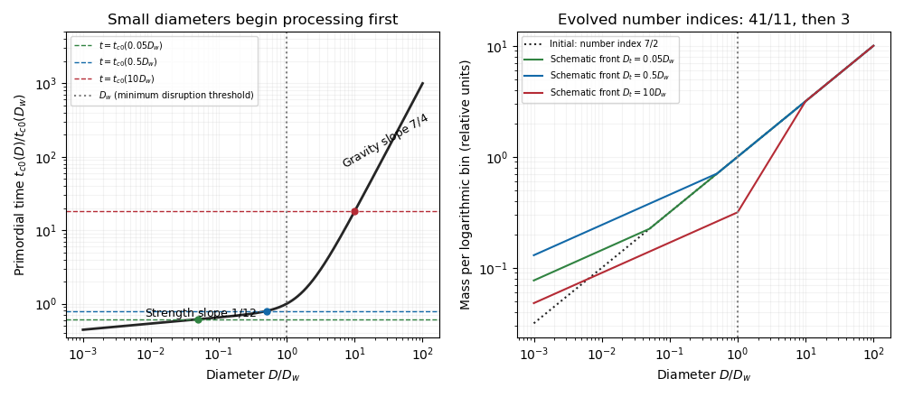
For the uniform depletion, the binary-collision evolution operator $F$ is quadratic in all bin masses: $F(cm)=c^{2}F(m)$. Let $m(t)$ be the undepleted trajectory and suppose $m_d(T)=m(T)/f$. Differentiating verifies the exact scaling within this fixed-kernel collision model,Immediately after depletion the shape is unchanged and the catastrophic planetesimal collision rates are reduced by $f$. Further evolution therefore proceeds $f$ times more slowly on the original trajectory. The processed-to-primordial transition initially remains at $D_t$, then advances on the stretched collision clock.

A collision-only model starting with the smaller initial normalization $m(0)/f$ has trajectory $\tilde{m}(u)=m(u/f)/f$. Matching the observed depleted distribution requires $u/f=T+(t-T)/f$. Hence the collisional age after uniform dynamical depletion isThe lower observed normalization would make it appear that slow collisions had taken much longer to produce the existing break. Shape and normalization alone cannot determine $f$ without independent information about age, initial mass, or depletion history.

Finally, count all impacts exceeding the strength threshold $Q_s=Q_a{D}^{-1/2}$, including impacts which also disperse the target. This is the source's inclusive rubblising convention; a bound-remnant rubblising collision alone would exclude the dispersing impacts. In the evolved gravity-regime projectile approximation, ${\alpha }_g=3$, so the given threshold-rate law gives the rubblising-to-dispersal collision-rate ratioAt the collisional front $D_t$, the age is of order one catastrophic collision time. Thus the expected number of strength-shattering impacts has the large-$D_t/D_w$ scalingThis is the requested scaling. It is not an exact unit-coefficient identity from the stated assumptions: using the true minimum diameter gives $R_{\mathrm{rub}}/R_{\mathrm{cc}}\simeq 3^{-2/3}(D_t/D_w{)}^{4/3}$. The actual cumulative number is ${\int }_0^T{R}_{\mathrm{rub}}(D_t,t)dt$, not automatically $T{R}_{\mathrm{rub}}(D_t,T)$, and its coefficient depends on evolution of the projectile population. The $4/3$ estimate also assumes the relevant projectiles sample the gravity-regime slope; sampling the strength or primordial slope changes the exponent. The steady-cascade framework and evolving transitions are developed by Wyatt, Clarke and Booth.

Radiative drag is only one of several loss mechanisms. Around a star, radiation-pressure blowout can eject small fragments; its $\beta =1/2$ threshold applies specifically to zero-kick release from a circular parent orbit. Stellar-wind drag and gas drag can drive planetary migration, while sublimation destroys grains approaching high-temperature regions. Collisional cascades destroy or fragment grains and can feed the unbound size range. Planetary scattering can cause ejection, collision with a planet, or a stellar impact; resonant trapping of dust can instead delay planetary migration.

For circumplanetary orbits, collisions with the planet or its satellites, disruption in collisions, and escape under stellar tidal forces are additional losses. Orbits near or outside the Hill sphere need not remain planet-bound. Radiation pressure on circumplanetary dust can excite planetocentric orbital eccentricity or unbind very small grains; it need not act only through slow Poynting–Robertson drag. For charged grains, the Lorentz force in stellar or planetary magnetic fields can alter or destabilize an orbit. Shadowing of circumplanetary dust changes the radiation-force average and can reduce the quoted decay rate. Which mechanism dominates depends on grain size and composition, environment, orbit orientation and the available collision or gas density.

For equal logarithmic width $d\log D$, the number of bodies is $n(D)Dd\log D$. Their mass is thereforeThe mass removed by catastrophic planetesimal collisions per logarithmic bin per unit time scales asAssume a steady collisional cascade with supply only at the large end, loss only at the small end, negligible reassembly or cratering contributions, and self-similar fragmentation that transfers mass through comparable logarithmic intervals. Mass conservation requires the downward mass flux across every intermediate size boundary to be the same; otherwise mass would accumulate or deplete there. Under the scale-invariant bin-transfer assumption, this is proportional by a size-independent factor to ${\dot{M}}_{\mathrm{loss}}$, soThis is constant mass flux in a collisional cascade. Steady state alone fixes the net flux, while the identification with the destruction rate of each bin additionally uses the stated fragmentation assumptions.

A size-independent $Q_D^{\ast }$ gives the steady Dohnanyi collisional cascade exponent $\alpha =7/2$. The preceding results becomeThus, under these idealized prescriptions, cratering collisions remove target mass about three times faster than catastrophic collisions. The conclusion concerns mass removed from targets; both processes contribute fragments to the collisional cascade.

If $Q_D^{\ast }\propto D^b$, part (b) givesThe mass in one logarithmic size interval scales as $D^3[Dn(D)]\propto D^{4-\alpha }$. A steady collisional cascade requires the mass destroyed per unit time, and hence the mass flux through every logarithmic interval, to be independent of $D$. Its exponent is thereforeSolving gives

When a loss mechanism becomes slow again at very small diameters, a depleted intermediate band can feed a lower-normalization collisional cascade. For size-independent strength the asymptotic collision-dominated slope returns to $-7/2$. In the local two-limit Yarkovsky removal model, matching gives $D_{-}\sim D_0^{8/5}{D}_{+}^{-3/5}$ and normalization ratio $K_{-}/K\sim (D_0/D_{+}{)}^{2/5}$. Coefficients depend on the collision kernel; a sharp join is only an asymptotic sketch.

A simplified collisional cascade tracks large objects $S$ and small fragments $F$. A fragment can disrupt a large object and multiply, while fragment–fragment collisions remove material. With $\dot{S}=-\kappa SF$ and $\dot{F}=\alpha SF-\beta F^2$, elimination of time gives a linear differential equation, $dF/dS-(\beta /\kappa )F/S=-\alpha /\kappa$. It has solution $F=C{S}^k-(\alpha /\kappa )S/(1-k)$ for $k=\beta /\kappa \ne 1$. Its maximum occurs at $F=(\alpha /\beta )S$; early exponential growth does not imply permanent exponential growth after the large-object reservoir is depleted.