Chirped pulse amplification

Chirped pulse amplification increases an optical pulse's energy while keeping its peak power lower during amplification: stretch the pulse, amplify it, then compress it. A chirp is a changing instantaneous frequency. Stretching separates the arrival times of different frequencies; pulse compression brings their contributions back together. The gain medium supplies energy, whereas the compressor concentrates the surviving energy into a shorter time.

Donna Strickland and Gérard Mourou demonstrated chirped pulse amplification at Rochester in 1985. Their experiment used an optical fiber, a regenerative amplifier and a diffraction grating compressor.^[ref]

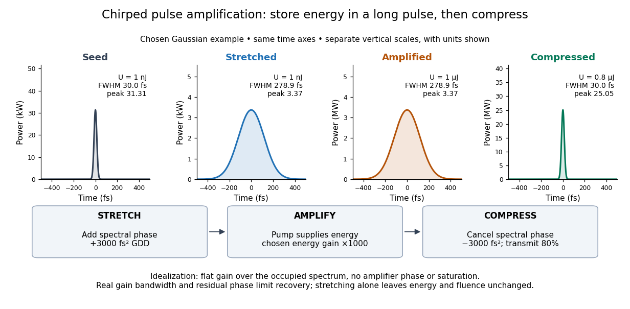
The useful idea is to arrange where the large peak power occurs. Lower light intensity in the amplifier reduces unwanted self-focusing and self-phase modulation; the compressed output can still drive strong nonlinear optics. Stretching does not remove every damage mechanism, and compression does not manufacture energy.

Let $P(t)$ be the pulse's power integrated over its transverse section, and $U$ its energy. Its peak power is ${\max }_{t}P(t)$. For a chosen Gaussian power envelope with full width at half maximum $\tau$,The numerical shape factor is approximately $0.9394$. It matters when comparing quoted peak powers; the estimate $U/\tau$ assumes a shape and a width convention.

If an otherwise unchanged pulse is stretched by a factor $S$ without loss, its energy stays fixed and its peak power falls by $S$. For energy gain $G$ and compressor energy transmission $\eta$, ideal restoration of the original shape givesThese relations require a specified shape and preserved spectrum; they do not model amplifier saturation. For the diagram's chosen $1\mathrm{nJ}$, $30\mathrm{fs}$ seed, $S=9.2959$, $G=1000$ and $\eta =0.8$, the successive peak powers are $31.31\mathrm{kW}$, $3.369\mathrm{kW}$, $3.369\mathrm{MW}$ and $25.05\mathrm{MW}$. The last pulse contains $0.8\mu \mathrm{J}$: the compressor increases peak power while losing some energy.

Fluence is time-integrated light intensity, $F(x,y)=\int I(x,y,t)dt$, measured in $\mathrm{J}{\mathrm{m}}^{-2}$. For a uniform beam of area $\mathcal{A}$, $F=U/\mathcal{A}$ and $I_{\mathrm{pk}}=P_{\mathrm{pk}}/\mathcal{A}$. At fixed transverse profile, lossless temporal stretching lowers peak light intensity but leaves fluence unchanged. Absorbed energy, heat removal, beam size, coatings and pulse duration still constrain optical components. For nonoverlapping identical pulses at repetition frequency $f_r$, the average power is $U{f}_r$; it is a different quantity from peak power.

Use a complex envelope $A(t)$ normalized so that $|A(t){|}^2=P(t)$; its units are ${\mathrm{W}}^{1/2}$. The optical carrier convention is $e^{-i{\omega }_{0}t}$: the physical electric field is proportional to the real part of $A(t)e^{-i{\omega }_{0}t}$ for a fixed transverse mode. With angular frequency offset $\Omega =\omega -{\omega }_0$, fix the Fourier transform conventionWrite $\tilde{A}=B{e}^{i\varphi }$ with real $B\ge 0$. A dispersive element adds spectral phaseConstant phase rotates the envelope; the linear term delays it by ${\varphi }_1$. The group delay is $d\varphi /d\Omega$. The quadratic coefficient ${\varphi }_2$ is group delay dispersion, abbreviated GDD, with units of time squared. Positive GDD makes higher frequencies arrive later with this convention. It is accumulated dispersion of a component; material group velocity dispersion is its corresponding coefficient per unit length.

To undo a quadratic stretcher spectral phase, the compressor must supply opposite GDD. Include the amplifier and all intervening optics in the sum:Setting this sum to zero does not cancel third-order dispersion, ${\varphi }_3$, or still higher orders. Residual spectral phase can produce asymmetry and satellite pulses even when the quadratic term vanishes. A diffraction grating system can make path length depend on frequency; matching the complete spectral phase over the occupied spectrum is more demanding than merely choosing opposite quadratic coefficients.

There is a useful proof of what phase correction can accomplish. By Parseval's identity,For a smooth decaying spectrum, the Fourier transform of $tA$ is $-id\tilde{A}/d\Omega$. Consequently the power-weighted mean arrival time and variance obeyAt fixed spectral amplitude, constant group delay minimizes this root mean square duration. Such a pulse is a transform-limited pulse, up to a time shift and constant phase. The nonnegative second term measures temporal broadening from unequal arrival times; the first term remains even after perfect phase correction.

Choose an initially transform-limited pulse with Gaussian power and complex envelopeHere ${\sigma }_0$ is the standard deviation of the power-weighted time distribution; ${\tau }_0$ is its full width at half maximum. Neither is a field-amplitude width. The spectral amplitude is proportional to $e^{-{\sigma }_0^2{\Omega }^2}$, so the spectral power has standard deviation ${\sigma }_{\Omega }=1/(2{\sigma }_0)$. The Gaussian time-bandwidth product in ordinary frequency is ${\tau }_0\Delta \nu =2\ln 2/\pi \simeq 0.4413$, where both widths are power FWHMs.

Multiplication by $e^{i{\varphi }_2{\Omega }^2/2}$ preserves spectral power and energy. Substituting ${\varphi }^{\prime }={\varphi }_2\Omega$ into the moment identity givesThis is an exact result for a Gaussian spectrum with quadratic spectral phase. It also follows by completing the square in its inverse Fourier transform.

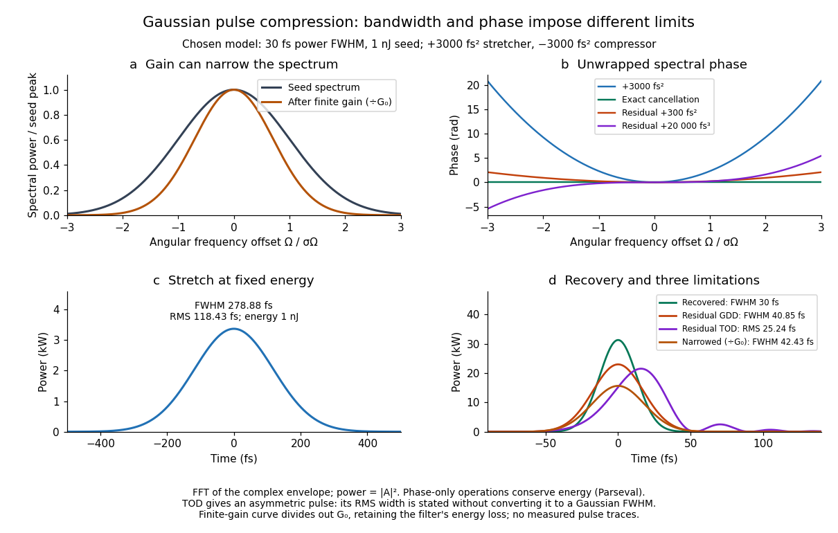
For these chosen inputs, ${\sigma }_0=12.7398\mathrm{fs}$. The stretched pulse has $\tau =278.88\mathrm{fs}$ and root mean square width $118.4282\mathrm{fs}$. Adding $-3000\mathrm{f}{\mathrm{s}}^2$ recovers $30\mathrm{fs}$; leaving $300\mathrm{f}{\mathrm{s}}^2$ gives $40.85\mathrm{fs}$. All phase-only cases retain $1\mathrm{nJ}$.

If GDD is cancelled but ${\varphi }_3=20000\mathrm{f}{\mathrm{s}}^3$ remains, the pulse is asymmetric. Gaussian spectral moments giveThus the centroid is $15.4033\mathrm{fs}$ and the root mean square duration is $25.2354\mathrm{fs}$. Converting this last value to a FWHM with the Gaussian factor would be wrong: the power envelope is no longer Gaussian. The calculation's integrated energy agrees in time and frequency through Parseval's identity, while its centroid and variance agree with these independent moment formulas.

A real amplifier also changes spectral amplitude. For a simple small-signal example, stipulate an intensity gain profileThis specifies finite gain bandwidth, with no saturation or extra amplifier phase. Multiplying two Gaussian spectra givesFor chosen ${\sigma }_g={\sigma }_{\Omega }$, the amplified spectrum is narrower by $\sqrt{2}$, the shortest Gaussian power FWHM becomes $30\sqrt{2}=42.43\mathrm{fs}$, and the total energy is $G_{0}U/\sqrt{2}$. Perfect spectral phase correction cannot recreate the suppressed spectral amplitude. Real gain narrowing and saturation require a material-dependent amplifier model; a constant multiplier is only a limited idealization. Gérard Mourou's 2018 lecture discusses gain narrowing as a limit on the shortest amplified pulses.^[ref]

The 1985 experiment launched $150\mathrm{ps}$ pulses from a mode-locked laser into $1.4\mathrm{km}$ of optical fiber. Dispersion and self-phase modulation produced a broader spectrum and approximately $300\mathrm{ps}$ pulses. A Pockels cell selected a pulse for repeated amplification in neodymium glass, giving approximately $2\mathrm{mJ}$ before the double-pass diffraction grating compressor. Its transmission was 50 percent. The amplified output was reported as $1\mathrm{mJ}$ with a $2\mathrm{ps}$ width limited by the streak camera response. The compressor was adjusted on fiber-output pulses using intensity autocorrelation; that measurement gave $1.5\mathrm{ps}$. Steve Williamson was acknowledged for help developing the concept, and Philippe Bado and Marcel Bouvier for technical support.^[ref]

The crucial comparison is compression before and after amplification. It asks whether enough usable spectral phase structure survives the amplifier, rather than merely whether its output is bright. A response-limited trace cannot establish the true width below the detector's resolution or prove that every higher-order phase coefficient vanished. An intensity autocorrelation is also not a direct unique measurement of the complex electric field. These are limits on the inference, not extra controls attributed to the experiment.

Donna Strickland's 2018 lecture describes setting the compressor with the high-repetition oscillator pulses and making the amplified-pulse measurement with Steve Williamson's streak camera. It explicitly notes imperfect chirp matching.^[ref] The first apparatus therefore illustrates the strategy without establishing a universal lossless or exactly phase-matched amplifier.

Donna Strickland leads an ultrafast laser group at Waterloo investigating intense laser interactions and nonlinear optics.^[ref] Gérard Mourou's later work includes coherent combination of laser beams in the XCAN project at École polytechnique.^[ref] Their complementary research settings connect the original short-pulse experiment with the continuing problems of producing useful energy, peak power and average power together.