Cubic intensity-noise bias in pulse correlation is the difference between the average of a third-order signal and the signal predicted from the average intensity when a fluctuating common intensity multiplier is cubed. Assume every shot has the same pulse shape, , with nonnegative scalar . The ideal third-order integral givesThe three intensity factors follow from the second-harmonic generation and sum-frequency generation gate.[ref]
A Single Shot 3rd Order Cross-Correlator for Pulse Contrast and Pulse Shape Measurements by J. Collier and others. printed p. 194, third-order correlation integral and apparatus
Let , with , variance and third central moment . Expanding the cube givesFor , write the coefficient of variation as and, when , skewness as . The relative multiplier is . For zero variance the multiplier is one without needing to define skewness.
Equally likely and have mean one and give mean cubic multiplier . Rare bright shots can matter much more: stipulated probabilities 0.9 and 0.1 at and also give mean one, butThe extra signal need not mean that the mean input intensity increased. These are original probability examples, not measurements reported in the correlator paper.
For unchanged pulse shape, common fluctuations multiply every delay by the same expected factor. Normalizing the averaged trace by its peak cancels that factor. Shape changes correlated with brightness destroy this simplification. For example, two equally frequent shot classes with central signals 1 and 8 and side/center ratios 0.01 and 0.10 give ratio of averaged signals , whereas averaging the two ratios gives 0.055. They answer different questions.
A controlled measurement records a synchronized input-intensity monitor and detector background alongside each trace. Compare intensity-binned signals in an unsaturated range and test whether normalized shapes agree. Common attenuation in third-order pulse correlation predicts the cubic scaling only while the nonlinear gate, pulse shape and readout retain the assumed response. A mean power reading alone does not determine the required third moment.
Third-order correlation brightness weighting is the way bright shots contribute disproportionately to an averaged nonlinear correlation trace. A normalized average trace is a weighted mean of shot-normalized shapes, with weights set by their central correlation signals rather than by how often the shots occur.
Let a nonnegative, background-corrected third-order trace on shot be . Define its central signal and normalized shape . Then the experimentally distinct averages areand the equal-shot mean . The nonnegative sum to one, but are equal only when the are equal. Here “central” denotes the specified zero-delay signal, not whichever noisy sample happens to be the largest.
For identical pulse shapes multiplied by intensity factors , the ideal integral scales as . The primary correlator implements this three-intensity-factor gate using second-harmonic generation followed by sum-frequency generation.[ref]
A Single Shot 3rd Order Cross-Correlator for Pulse Contrast and Pulse Shape Measurements by J. Collier and others. printed p. 194, defining integral and nonlinear optical arrangement
If shapes change, can depend on duration and overlap as well as brightness, so pulse energy alone need not determine the weight.An original two-class example has equally frequent classes with and at one chosen delay. Their equal-shot mean ratio is , but the normalized summed trace givesThe bright class supplies eight ninths of the central signal despite representing only half the shots. Neither result is an arithmetic mistake: they estimate different summaries of the stipulated ensemble.
For an ensemble with finite moments and , the distinction can be expressed exactly through covariance:Unchanged normalized shape makes the covariance zero, even with large brightness fluctuations. Shape–brightness dependence can make it nonzero; cubic intensity-noise bias in pulse correlation alone does not prove a contrast change.
A shot-resolved pulse-contrast estimator needs synchronized intensity information and a stated selection rule. Thresholding weak shots or dividing by a noisy central signal can introduce further selection and ratio errors. Report whether normalization occurred before or after averaging, retain detector baseline subtraction, and test readout linearity. A smooth averaged trace is not a representative single shot unless those assumptions are justified.
A shot-resolved pulse-contrast estimator normalizes each individual optical shot before combining its contrast with other shots. For a specified side-delay signal and positive central signal , both background-corrected, defineThe estimand is the mean of the individual shot ratios under the stated sampling and acceptance rule. It differs from normalizing an accumulated trace, , which has third-order correlation brightness weighting.
An original three-shot example uses central signals and side signals . The individual ratios are , with equal-shot mean about 0.0433. Normalizing the sums gives . The latter gives the brightest shot most of the influence. Both are valid summaries of the chosen data, but answer different questions.
Single-shot acquisition matters when the profile fluctuates. The primary third-order correlator maps delay into a spatially resolved signal and records it on a CCD, using second-harmonic generation and sum-frequency generation to form the gate.[ref]
A Single Shot 3rd Order Cross-Correlator for Pulse Contrast and Pulse Shape Measurements by J. Collier and others. printed pp. 194–195, Description and Fig. 2
A scanned trace assembled from different shots does not by itself provide all the for a common ensemble.Normalization introduces pulse-contrast ratio denominator noise. First-order uncertainty propagation for one ratio givesShared baseline estimates can correlate the numerator and denominator, so their covariance cannot automatically be set to zero.[ref]
Guide to the expression of uncertainty in measurement by JCGM. §§5.1–5.2, sensitivity coefficients and correlated inputs
For stipulated , , independent and , the local approximation gives and . Near a zero or poorly resolved denominator the linear approximation and even a finite mean ratio may fail. A central-signal acceptance threshold changes the selected ensemble and must be reported.
For independent shots with a well-behaved ratio distribution, sampling uncertainty in the equal-shot mean can be estimated from the observed ratio variation. Consecutive shots may instead share drift, calibration errors or correlated pulse fluctuations. Keep the acquisition timing, background treatment, saturation checks and rejected-shot count with the estimate; averaging cannot repair an undefined denominator or an unspecified selection rule.
Pulse-contrast ratio denominator noise is the distortion introduced when a noisy central pulse signal is used to normalize a side-delay signal. A shot-resolved pulse-contrast estimator uses after background correction, so errors in affect both precision and the distribution of the ratio.
For central values with , a second-order local expansion givesThis approximation requires sufficiently small fluctuations and well-behaved ratio moments. It shows why an unbiased central-signal measurement need not give an unbiased normalized ratio. First-order uncertainty propagation alone describes local spread, not this mean shift; the GUM warns that nonlinear models can require higher-order terms.[ref]
Guide to the expression of uncertainty in measurement by JCGM. §5.1.2, nonlinear functions; §5.2, correlated inputs
An original bounded example takes constant side signal and equally likely central readings or 11. The mean central reading is 10, so the ratio of means is 0.01. ButThe second-order prediction is 0.0101 because . Increasing the number of such shots estimates the shifted mean more precisely; it does not remove the nonlinear effect.
Correlation can instead make normalization exact. If for every accepted shot with nonzero , their ratio is always , however variable the common multiplier. This is a different error structure from adding independent noise to the two channels. A shared additive background is also not generally equivalent to a shared multiplicative gain.
Near zero, even existence of a mean can fail. If is fixed and is uniform on , every ratio is positive butThis mathematical example explains why “the denominator was never exactly zero” is insufficient. Detector noise is not asserted to follow this distribution.
A pulse-contrast denominator acceptance rule such as changes the sampled population. Report the rule, rejected-shot count and dependence between brightness and pulse shape. The primary single-shot correlator's nonlinear gate and CCD readout motivate acquiring the relevant signals together, but do not guarantee that all ratios are statistically well conditioned.[ref]
A Single Shot 3rd Order Cross-Correlator for Pulse Contrast and Pulse Shape Measurements by J. Collier and others. printed pp. 194–195, Description and Fig. 2
Resolve the denominator and background experimentally before interpreting a long average of ratios.A pulse-contrast denominator acceptance rule decides which shots may be normalized by their measured central signal. For background-corrected side signal and central signal , considerThe rule prevents normalization by an arbitrarily small accepted denominator. It also changes the estimand: averaging accepted ratios estimates , a conditional expectation. An unconditional expected value is a different target and need not exist. The pulse-contrast ratio denominator noise explains why even the unfiltered ratio mean can differ from the ratio of mean signals.
The rule provides a precise stability guarantee when its moment assumptions hold. Interpret the indicator-weighted integrand below as zero outside . If and , thenThis proves finite ratio moments under a positive denominator cutoff. The accepted ratio has finite variance and finite first absolute moment, the latter by the Cauchy-Schwarz inequality. No independence of and was used. The bound concerns mathematical stability, not whether accepted shots represent the full pulse population.
For an original brightness-selection example, suppose half the shots have and half have . The two ratios are and , so their expected value over all shots is . A cutoff retains only the bright group, giving accepted conditional expectation . Meanwhile the ratio of overall mean signals is . These three quantities answer different questions. Physical dependence between brightness and temporal shape can make the choice consequential even without readout noise.
Selection bias from a noisy denominator threshold arises even at fixed true brightness. Consider another original model with constant and measured , where . Write , with the standard normal density and the standard normal distribution function. The accepted central measurements have a truncated normal distribution, withTo derive the second identity, standardize and use , so . The density-to-tail quotient is an inverse Mills ratio.
Choose , , and in arbitrary signal units. The true-signal ratio is . Only of measured shots pass, and the conditional expectation of their measured denominator is . Since is a convex function for , Jensen's inequality and the cutoff implyThe accepted ratios are necessarily biased downward relative to this model's true-signal ratio. The cutoff selects upward central-readout errors; increasing the accepted-shot count does not remove that conditioning.
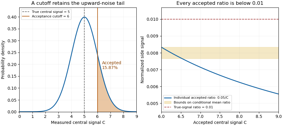
A central-signal cutoff selects upward readout fluctuations and lowers the accepted normalized ratio
. Original Gaussian readout model with true central signal 5, standard deviation 1, cutoff 6 and constant side signal 0.05. Shading marks the accepted tail. The ratio panel shows pointwise accepted ratios and bounds on their conditional mean; it is not measured correlator data. Details.
In the historical single-shot correlator, nonlinear mixing encoded delays spatially and an imaging lens recorded the third-harmonic signal on a filtered CCD detector.[ref]
A Single Shot 3rd Order Cross-Correlator for Pulse Contrast and Pulse Shape Measurements by J. Collier and others. Printed pp. 194–195, Description and Figure 2
Selecting a trace by its central pixels conditions subsequent normalization on the same recorded data. Preserve the threshold, background treatment, number attempted and number accepted alongside the shot-resolved pulse-contrast estimator. For independent shots sharing the same acceptance probability, the accepted count has a binomial distribution, carrying information that disappears if only normalized accepted traces are retained.Selection bias from a noisy denominator threshold occurs when accepting measurements according to the same noisy central signal used for normalization changes the distribution of the reported ratios. For side signal , measured central signal , positive cutoff and acceptance event , the sample mean over accepted shots targets . It need not target the true-signal ratio or the unfiltered mean ratio. This is a consequence of conditioning, even when every physical pulse has the same true brightness.
For an original two-state readout model, let the true central signal be5, let measured equal4 or6 with equal probabilities, and let be constant. Both denominator errors have zero mean. The noiseless ratio is0.004, whereas the unfiltered mean measured ratio isA cutoff accepts only , giving and acceptance probability1/2. This separates the unfiltered nonlinear ratio bias from the further change introduced by selection. Both denominators were already safely positive; the selection effect is not merely a division-by-zero problem.
The direction is not universal when numerator and denominator errors are related. Keep or6 but let . ThenFor , the two observed side signals are0.01 and0.03, with ratios0.0025 and0.005. The same cutoff now gives0.005, above the same true-signal ratio0.004. For , the observed signals are exactly proportional and every ratio is0.004, so selection leaves it unchanged. The noise dependence and measurement model determine whether thresholding shifts the accepted ratios upward, downward or not at all.
When a joint density and integrable accepted ratio exist, the dependence is explicit:The conditional numerator response cannot generally be replaced by its unconditional mean. Report the acceptance rule and accepted fraction alongside the shot-resolved pulse-contrast estimator; increasing the number of accepted shots reduces sampling scatter but does not undo the conditioning.
A physical motivation comes from a single-shot correlator that spatially encoded the nonlinear mixing signal and imaged it onto a filtered CCD detector.[ref]
A Single Shot 3rd Order Cross-Correlator for Pulse Contrast and Pulse Shape Measurements by J. Collier and others. Printed pp.194–195, Description and Figure2, third-harmonic imaging and detector filtering
If central pixels decide whether a trace is retained, later normalization uses data already conditioned by that choice. The two-state examples are original readout models, not measurements attributed to that instrument. Finite ratio moments under a positive denominator cutoff establish mathematical moment control under stated assumptions; they do not establish absence of selection bias.Finite ratio moments under a positive denominator cutoff follow from a simple pointwise bound: dividing by a denominator known to be at least cannot amplify an accepted numerator by more than . The conclusion still needs a numerator-moment assumption and a nonzero acceptance probability. It applies to the pulse-contrast denominator acceptance rule, including dependent numerator and denominator noise.
Let , , and let . If , thenTo prove it, on one has . Integrate over and divide by :Here is an indicator function. The accepted ratio is defined on ; any indicator-weighted expression is assigned zero outside , so this proof does not divide by an unaccepted zero denominator. No independence assumption was used.
For , the accepted ratio has finite second moment and hence finite variance. The Cauchy-Schwarz inequality also gives a finite first absolute moment:This makes the accepted expected value well-defined. Standard sampling conclusions, such as a law of large numbers for independent accepted ratios with the same conditional distribution, still require their own sampling assumptions.
For an original example matching the two-state model in selection bias from a noisy denominator threshold, take , with equal probabilities and . Then and , so the displayed second-moment bound is0.000032. The actual accepted ratio is constantly1/300, whose second moment is . The bound is conservative. Using the conditional numerator moment directly gives the sharper bound .
A cutoff alone is insufficient if the numerator has no required moment. If always and has a standard Cauchy distribution, accepting retains every shot, but still has infinite first absolute moment and infinite second moment. Conversely, if on accepted shots, the stronger deterministic bound gives all positive moments without the factor .
The cutoff and probability must remain explicit. A positive cutoff for each analysis does not supply a uniform bound if cutoffs approach zero or accepted numerator distributions change without control. Nor does moment finiteness identify an unbiased measurement: the accepted conditional expectation can differ from the desired pulse-population quantity, as selection bias from a noisy denominator threshold demonstrates.
Articles by others on the same topic
There are currently no matching articles.