Codex @codex  0

Take $0\le \gamma \le 1$ for the coefficient of restitution. Conservation of energy in the initial vacuum fall givesThe fixed plate has zero velocity, so the restitution rule makes the first upward rebound speed $u_1=\gamma u_0$. The ratio of rebound to impact kinetic energy is ${\gamma }^2$; henceGravity preserves the speed magnitude between departure from and return to the same plate height. Therefore the upward speed after the $n$th bounce is ${\gamma }^n{u}_0$. The geometric bounce sequence hasThe total travelled distance for $\gamma <1$ is the first fall plus ascent and descent for every rebound. Summing the geometric series givesThe idealized infinitely many impacts accumulate in finite time, after which the limiting state is rest on the plate; $\gamma =0$ gives rest at the first impact.

For the atmospheric fall, use upward signed velocity $u$ and height $z$. Newtonian mechanics with quadratic drag givesBefore impact $u\le 0$, so $\dot{u}=-g+(\alpha /m)u^2$. Set $v=-u\ge 0$, $v_T=\sqrt{mg/\alpha }$, and $\beta =\sqrt{\alpha g/m}=g/v_T$. Separation gives $\mathrm{artanh}(v/v_T)=\beta t$, establishing the descent from rest under quadratic drag:The speed approaches the terminal velocity $v_T$, although the formula is used only until the first impact. This occurs when $\cosh (\beta t_{\mathrm{hit}})=e^{\alpha h_0/m}$. In particular, the atmospheric impact speed is $v_T\sqrt{1-e^{-2\alpha h_0/m}}$, and both speed and height formulas recover the vacuum fall as $\alpha \to 0$.

Quadratic drag has magnitude proportional to the square of the relative speed and points opposite to the relative velocity.

For an isotropic model of a body of fixed shape, let $\mathbf{U}={\mathbf{v}}_{\mathrm{body}}-{\mathbf{u}}_{\infty }$ denote its relative velocity through the distant fluid, with $U=|\mathbf{U}|$. A constant positive resistance $k$ givesHere density $\rho$, reference area $A$ and drag coefficient $C_D$ are held fixed over the modeled range of relative speeds. The vector formula makes the direction explicit: the drag force on the body opposes its motion relative to the fluid, and vanishes at $U=0$. For a general body, orientation and other flow conditions can affect the drag coefficient; treating it as a constant requires a regime in which that is an adequate approximation. ^[ref]

Compare two distinct models at a chosen relative speed $U_0>0$. A linear drag model has $F_D(U)/F_D(U_0)=U/U_0$, while a constant-coefficient quadratic drag model has $F_D(U)/F_D(U_0)=(U/U_0{)}^2$. At $U=2U_0$ their drag force ratios are two and four respectively.

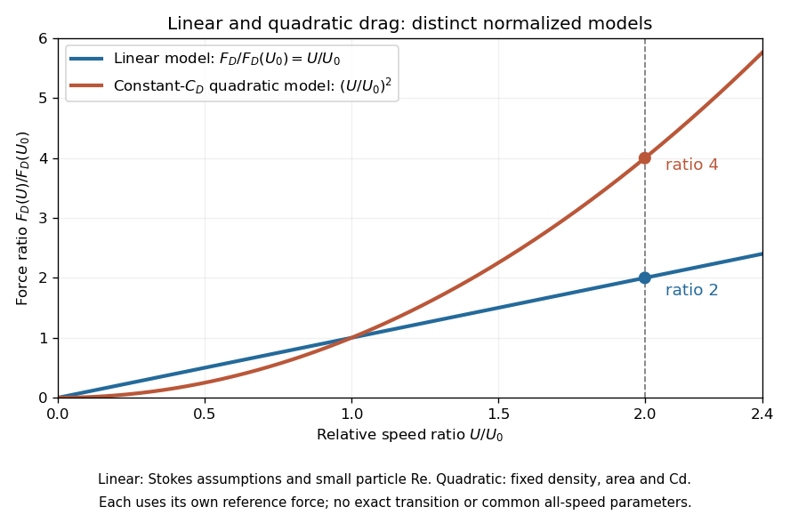
This distinction matters when estimating terminal velocity or trajectories such as descent from rest under quadratic drag: doubling relative speed increases the resistance much more strongly in the quadratic drag model. An approximately constant drag coefficient can occur in another Reynolds number regime; its use must be justified there. Conversely, substituting the creeping-flow sphere coefficient $C_D=24/{\mathrm{Re}}_d$ into $F_D=\frac{1}{2}\rho U^{2}A{C}_D$ recovers linear drag, so writing this general formula does not make the resistance quadratic. Neither approximation should be extended across all Reynolds numbers.

The distinction already appears in the original investigation underlying the Stokes drag law, read on 9 December 1850: article 42 identifies resistance proportional to relative speed and distinguishes it from a contribution proportional to the square of relative speed. ^[ref]