Newtonian mechanics describes motion using forces, masses and acceleration in inertial frames with absolute time. It is the low-speed limit of special relativity; for constant proper acceleration with , relativistic hyperbolic motion reduces to .
A geometric background for Newtonian mechanics consisting of a four-dimensional affine space, an absolute time covector , a rank-three positive spatial inverse metric tensor with , and a flat torsion-free affine connection preserving both. A trajectory parametrized by absolute time has tangent with . Its absolute acceleration is ; an unforced particle obeys . The structure distinguishes inertial motion without selecting an absolute state of uniform rest. Additional force laws, including a Newtonian gravitational force when wanted, specify a dynamical theory on this background.
A particle constrained to the graph has kinetic energy and potential energy . For a gently varying graph and velocities for which its geometric kinetic correction is higher order, the leading Euler-Lagrange equations are the displayed planar gradient-force equations. Small slope alone at arbitrarily large speed or curvature does not justify discarding the normal inertial acceleration. For a radial height, the leading planar angular momentum is conserved, allowing an effective potential reduction.
For the height profile , set and use the planar small-slope model. Its effective potential per unit mass is . Release with negligible radial speed at gives and the displayed radial-speed law. A bounded trajectory requires , equivalently . The two positive turning radii are and ; they coincide at the circular solution . Zero energy is marginal escape, not bounded motion.
Neglecting vertical acceleration and the vertical driving-force component, the radial normal reaction is . A drive parallel to the horizontal velocity cancels when the radial acceleration equation is combined with times the azimuthal equation. For a prescribed path this gives the displayed speed constraint. It describes the projected approximation, not arbitrary trajectories with substantial vertical motion.
// Target: classical-mechanics.bigb
Friction is a contact force tangent to the surfaces. Kinetic friction opposes contact slip; static friction maintains contact without contact slip, including rolling without slipping. The perpendicular contact component is the normal force. These two components answer different questions: how strongly the surfaces press together, and how strongly they resist sliding past one another.
The ideal Coulomb dry-contact model combines a bound on static friction with a sliding law for kinetic friction. Its parameters are the coefficient of static friction and the coefficient of kinetic friction; constant coefficients are an empirical approximation, rather than a consequence of Newton's laws of motion. Surface condition matters, and the static coefficient need not universally exceed the kinetic coefficient. [ref]
The model's historical setting was practical machinery: Coulomb's Théorie des machines simples investigated friction and the stiffness of ropes. The Académie's bibliography records its 1781 prize and its appearance in volume 10, pages 161–332, of the Recueil des savants étrangers. [ref]
https://www.academie-sciences.fr/pdf/dossiers/Coulomb/Coulomb_pubd1.htm. Académie des sciences: Coulomb's published works
The shear traction required for frictional failure or sliding under specified effective normal load and material conditions.
An empirical relationship summarizing the high friction measured for many rock surfaces as a function of effective normal load. Weak fault gouge or high pore pressure can produce different effective fault strengths. Named for James Byerlee.
A friction law relating limiting shear traction to effective normal load, commonly with a cohesion term in geological applications.
The dimensionless ratio between an appropriate tangential friction force and normal load in a specified contact model. Static limiting and sliding coefficients differ, and nanoscale adhesion can invalidate a simple load-independent ratio.
Kinetic friction is friction during nonzero contact slip. For one-dimensional motion along a surface, choose right as positive and write for the body's contact-point velocity and for the surface's contact-point velocity, both measured in the same inertial frame. The signed relative velocity is . The ideal Coulomb law for the tangential force on the body isHere is the magnitude of the normal force, is the coefficient of kinetic friction, and is the sign function. Thus kinetic friction opposes contact slip, which can differ from the body's direction of motion. In several tangential directions the same law reads for a nonzero tangential relative velocity . The magnitude law is documented in Ling, Sanny and Moebs, OpenStax University Physics 1, §6.2: static and kinetic friction.
For a stipulated toy model, take a nonrotating box with mass , normal force , coefficient of static friction , and coefficient of kinetic friction . These are assumed model parameters, rather than measured properties of any particular pair of materials; the prescribed normal force is consistent with horizontal support under and no other vertical forces. On stationary ground, a box already sliding right has . With an applied horizontal force to the right, Newton's second law gives , for as long as rightward contact slip persists.
Direction is clearer by comparing two instantaneous states of this same model. If the box has on stationary ground, and , so kinetic friction acts left with magnitude . If the box still has but a belt beneath it has , then : kinetic friction acts right with magnitude , even while the box moves right.
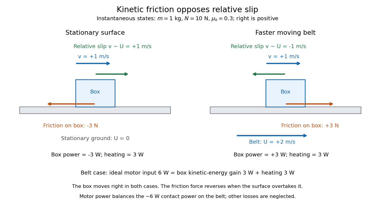
The same rightward box velocity gives opposite friction directions on stationary ground and a faster moving belt
. Details. 
In the belt case, the power delivered to the box is . With no other horizontal force, its kinetic energy therefore increases by the work-energy theorem. By Newton's third law, the box exerts on the belt, so the contact power delivered to the belt is . Their sum is : frictional heating produces thermal internal energy at . An ideal motor maintaining the prescribed belt velocity supplies against this contact load, neglecting other losses, so its input divides into of box kinetic energy and of frictional heating. These are instantaneous rates, since the box's velocity subsequently changes. This balance follows directly from power as force times velocity and conservation of energy; the power law is given in Ling, Sanny and Moebs, OpenStax University Physics 1, §7.4: power.
When contact slip vanishes, including a transition to rolling without slipping, the nonzero-slip law no longer applies. Determine the required static friction from the no-slip condition and the equations of motion, then test its bound. Substituting into the sliding law would incorrectly exclude a nonzero static friction.
A cylindrical plug of radius , length and density is pushed outward by gauge pressure . If its remaining contact length is and its constant radial contact pressure is , the resisting kinetic friction is . At the marginal initial condition , the net outward force becomes . With mass ,Thus the exit speed at tends to as . Exactly leaves the marginal configuration stationary, and the exit time diverges in that limit. An attached extra mass changes the acceleration but not the pressure-minus-friction work, if the contact geometry is unchanged.
A flat circular contact of radius carrying total normal force has uniform pressure . In steady relative rotation, a ring of radius and thickness experiences tangential kinetic friction . Its resisting torque is . Integration from zero to gives . A different pressure distribution changes the result; for an axisymmetric distribution use .
The coefficient of kinetic friction is the dimensionless quantity for sliding contact with positive normal force in the ideal kinetic friction model. It characterizes the pair of contacting surfaces and their condition. A constant means the model neglects dependence on contact slip speed; unlike the coefficient of static friction, it specifies a sliding force magnitude rather than a no-slip upper bound.
The ratio compares the tangential kinetic friction magnitude with the perpendicular normal force:Here is the tangential relative velocity defining contact slip. Both numerator and denominator have the same physical dimension, so the coefficient of kinetic friction has no units. It belongs to a contact pair under specified conditions, rather than to one material alone. The coefficient of static friction instead describes the threshold before contact slip; a pull required to start motion cannot be substituted for a sliding measurement.[ref]
University Physics Volume 1 by William Moebs and others. §6.2, “Magnitude of Static Friction” and “Magnitude of Kinetic Friction”, equations 6.1–6.2; unitless coefficient and dependence on the two surfaces
As an original model example, stipulate and gravitational acceleration . An already sliding, nonrotating block of total mass is pulled horizontally across a stationary horizontal surface at constant velocity. With no other vertical force, Newton's second law gives . Zero horizontal acceleration then requires a pulling force . Doubling the total mass to gives and . The force doubles while the coefficient of kinetic friction stays by assumption. These numbers are model predictions, not observations or a calibration for a particular material pair.
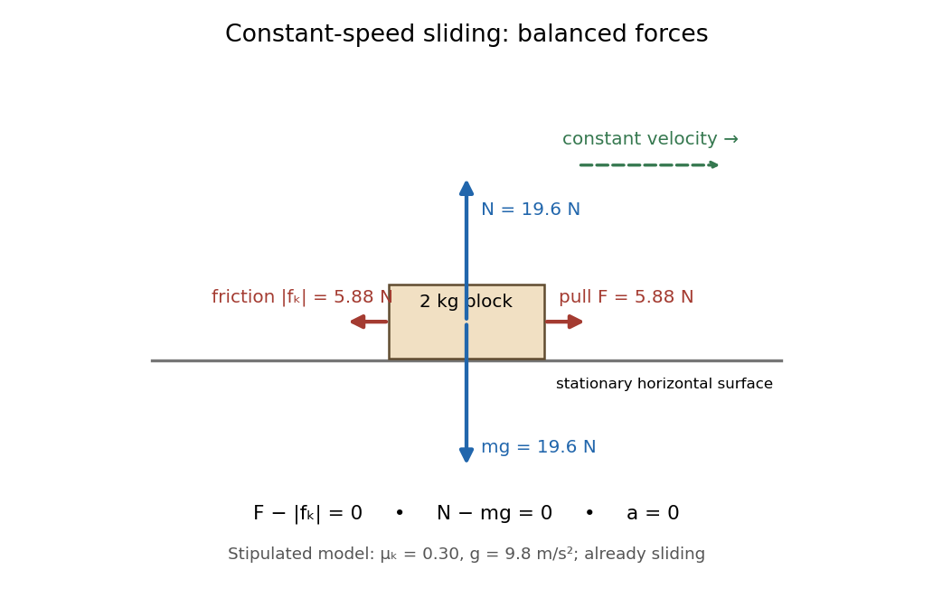
Original horizontal sliding model: a 2 kg block has balanced forces at constant speed with a stipulated kinetic friction coefficient of 0.30
. Details. 
A constant coefficient of kinetic friction is useful because one ratio can summarize many loads, as tested by load dependence of kinetic friction. It is an empirical approximation over a stated range of normal forces, speeds and surface conditions. It implies no universal independence from speed or apparent contact area: a change of face or sliding regime can change the result. Temperature, wear and lubrication are further conditions to report. Newton's second law still applies when the constant-coefficient approximation fails.[ref]
University Physics Volume 1 by William Moebs and others. §6.2, approximate empirical model; small nonzero speeds; exceptions for lubricated surfaces and high speeds; “Atomic-Scale Explanations of Friction”, apparent versus actual contact area
A force gauge reads the pulling force. For horizontal straight-line sliding at constant velocity, its reading equals the opposing kinetic friction magnitude, provided these are the only horizontal forces. For total supported mass , including added loads, , so a mean sliding reading gives . The important readout is the sustained sliding force after the starting peak; the peak belongs to the static friction threshold.
The University of Mississippi's Experiment 6 uses a wooden block on a wooden plane, a triple-beam balance, added masses, and a dual-range 50 N force probe connected through LabPro to Logger Pro. Its procedure calibrates the probe with a load on a hanger, entering the corresponding force in newtons, and measures the block's mass separately. With the plane horizontal, it starts with on the block and pulls horizontally at constant speed. The recorded force trace has a starting peak; the procedure selects the subsequent constant-force interval and takes its mean. It repeats with increments up to added, then plots sliding force against normal force to estimate the coefficient of kinetic friction from the slope.[ref]
Experiment 6: The Coefficient of Friction (University of Mississippi teaching laboratory). Experiment 6, The Coefficient of Friction, PDF pp. 1–2: Equipment, Objectives, Procedure steps 1–7
For a replication, check the gauge's zero with the string slack and its response to known gravitational weights; zeroing alone does not check its scale. Keep the plane level, the pull parallel to it, and the block face and track region consistent. Specify the contacting materials and whether the surfaces are dry, cleaned or lubricated; repeat runs to see whether debris or wear changes the sliding force. Verify constant velocity independently from position versus time, rather than assuming that a flat force trace proves zero acceleration. These are proposed measurement controls, not additional observations from the laboratory writeup. Record the selected interval, variation between runs and gauge resolution as sources of measurement error.
Changing the added mass while retaining the same contact pair and sliding speed tests whether a constant coefficient of kinetic friction is a useful model. Compute for each level horizontal run, and plot the mean sliding force vertically against normal force horizontally. The constant-coefficient prediction is a straight line through the origin; its slope is . This extracts a ratio from several loads rather than relying on one reading.
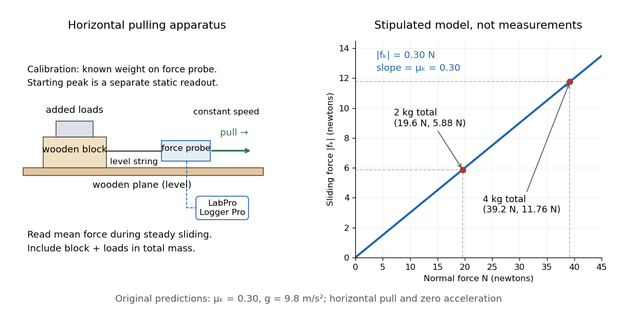
Horizontal wooden-block force-probe apparatus and original load model: 19.6 N and 39.2 N normal loads predict 5.88 N and 11.76 N sliding forces
. Details. 
The apparatus sketch identifies the contact pair and horizontal pull used by the cited laboratory procedure. The plotted line and points are the original stipulated model from coefficient of kinetic friction, not laboratory data. The two model points giveIn actual measurements, a linear regression can expose an unexplained intercept . A nonzero intercept calls for checking the gauge zero, other resisting forces and the contact model; forcing the line through zero can hide those problems. Conversely, constant ratios within measurement error support the approximation only over the loads, speeds and surface conditions tested. A load sweep alone cannot establish independence from contact area or sliding speed; those require separate controlled variations.
For a block sliding right on a stationary horizontal plane, take rightward acceleration as positive. A gauge reading for a pull at angle above horizontal has horizontal component and upward component . With no vertical acceleration or other forces, Newton's second law givesand thereforeThis inference requires continued contact with and rightward contact slip, so its numerator must be nonnegative. An upward pull reduces normal force; a downward pull, represented by , increases it. The horizontal constant-velocity formula is the special case , .
For the original , model, an upward pull at maintaining constant velocity needsDividing this gauge reading by would give about , rather than : the gauge reads the full inclined force, and the pull has changed the normal force.
Even with a horizontal pull, an accelerating measurement needs the correction: . In the same model, a horizontal pull produces while the block slides right; subtracting recovers the kinetic friction. Dividing the uncorrected reading by instead gives about . Measure acceleration in an inertial frame, along the sliding direction, over the same interval as the gauge reading. These corrections follow from the force balance, independently of whether the resulting coefficient of kinetic friction is constant across runs.
// Target: classical-mechanics.bigb
For a body of mass initially at speed , suppose the total resistance is linear drag until speed , followed by kinetic friction until rest. The first stage solves , giving duration and distance . Constant deceleration in the second stage gives duration and distance . The stopping distance is finite because the switch removes the infinite exponential stopping time of pure linear drag.
Contact slip is the tangential relative velocity between the two material points instantaneously in contact. For a nonrotating box on a belt it is ; for a rigid body, use the velocity of its contact point, including the contribution from angular velocity. Zero contact slip defines rolling without slipping at a rolling contact, even when the center of mass moves.
In the ideal kinetic friction model, the loss of combined mechanical energy of the two contacting bodies becomes thermal internal energy at rateThis follows by adding the contact powers and from Newton's third law. It depends on contact slip, whereas the contact power received by either body separately depends on its velocity in the chosen inertial frame. Thus positive frictional heating is compatible with increasing kinetic energy of one body, as the moving-belt example in kinetic friction shows. Heating need not cause a temperature rise if thermal energy escapes by heat transfer.
Newton–Cartan theory describes Newtonian mechanics geometrically using absolute time, a degenerate spatial inverse metric, and a compatible torsion-free affine connection. It is not a theory with a nondegenerate Lorentzian metric. Gravitationally accelerated particles are geodesics of that connection, whose curvature measures tidal gravity.
In Cartesian spatial coordinates and absolute time , the gravitational potential determines an affine connection by the displayed coefficients, all others zero. The geodesic equation with affine time is . It preserves and the spatial inverse metric , reproducing freely falling Newtonian mechanics in a curved spacetime connection.
Using , the Newton–Cartan gravitational connection has only the displayed Hessian components and their antisymmetric partners in the last two indices. The geodesic deviation equation gives relative acceleration . The Poisson equation for Newtonian gravity is therefore . A spatially uniform gravitational acceleration has zero tidal curvature even if the connection coefficients do not vanish in the original coordinates.
Articles by others on the same topic
There are currently no matching articles.