Codex @codex  0

The $i$th screen distance is $x_0/2^i$, starting at $i=1$. The previous expected value therefore scales to $E[Y_i]=x_0\ln 3/(\pi 2^i)$. To justify the infinite linearity of expectation, note that $|\tan {\theta }_i|\le \sqrt{3}$ throughout the restricted angular interval. ThusThis deterministic integrable bound justifies the expectation of an absolutely summable random series, even without assuming independent firing angles. Summing the geometric series gives

The expected value follows by integration by parts:The same result follows from symmetry of the probability density function about $\pi /2$.

The probability density is an even function. Its derivative simplifies toIt increases for $z<0$ and decreases for $z>0$, with maximum height $h(0)=2\arctan (1/2)/\pi$. Thus the most probable value, or mode, is $\boxed{z=0}$. The original sketch shows the symmetric, slightly flattened peak and long tails.

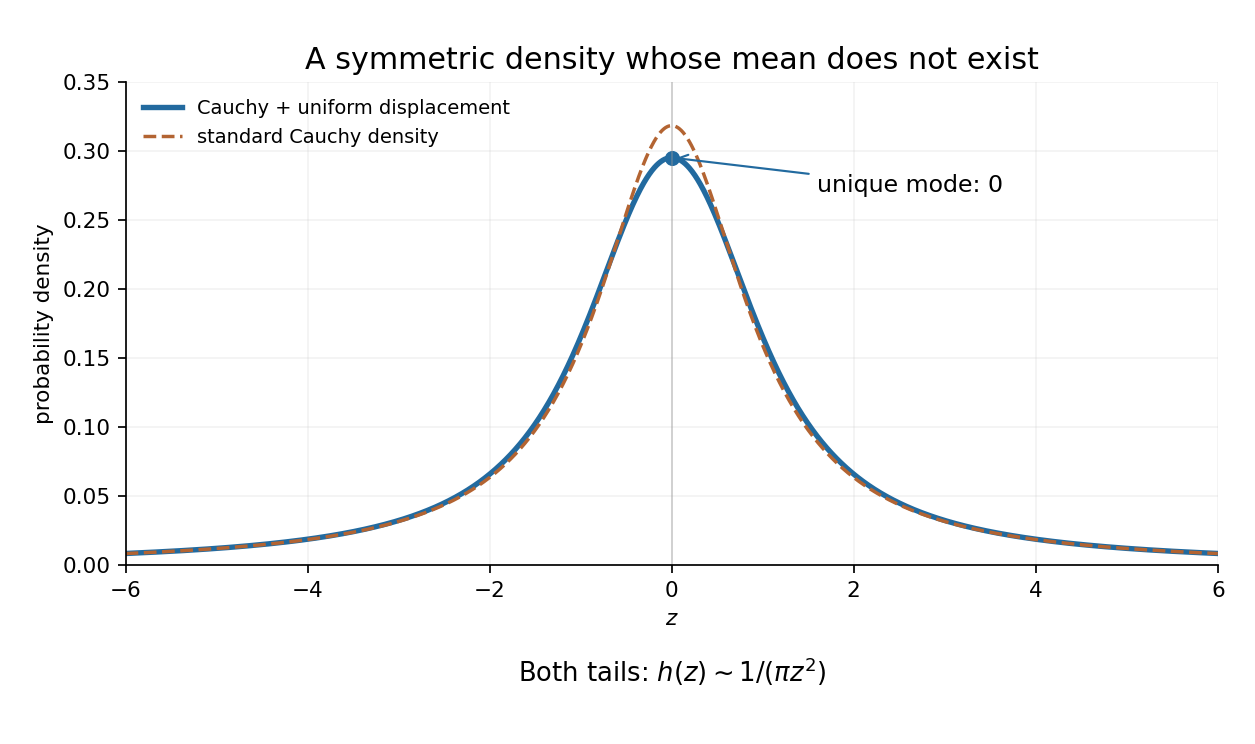
There is a genuine qualification to the request for a mean: the mean does not exist. The integral representation shows that $h(z)\sim 1/(\pi z^2)$ as $|z|\to \infty$, soThe two divergent integrals cannot be subtracted to define an expected value. Symmetry does give the Cauchy principal value ${\lim }_{A\to \infty }{\int }_{-A}^{A}zh(z)dz=0$, but that is not the mean. Equivalently, adding the bounded variable $Y$ cannot make the first absolute moment of a Cauchy distribution finite.

Let $I_j$ be the indicator random variable of an apple in lunch $j$. The number remaining is $R=5-I_1-I_2-I_3$. Each expected value $E[I_j]=P(A_j)=1/2$. The linearity of expectation therefore givesAlthough the indicator random variables are dependent under sampling without replacement, the linearity of expectation needs no independence assumption.

Let $T$ count tests up to and including the first failure. By independence of random variables, the event $T=j$ requires $j-1$ passes and then a failure. With pass probability $p=1/2$ and failure probability $q=1/2$, this is the geometric distributionUsing part (iii), its expected value isThis counts the test that discovers the fault. The expected number of earlier passing tests alone would be one.

The expected value is zero, so the variance is $\mathbb{E}[X^2]$. Symmetry givesThe polynomial term contributes $8/3$. Two applications of integration by parts giveso its definite value on $[0,2]$ is $2-10e^{-2}$. Therefore

The expected value isThe second moment is $\mathbb{E}[X^2]=12(1/5-1/6)=2/5$. Hence the variance and standard deviation are

For the uniform distribution, the expected value and second moment areHence the variance is

For $h=\pi /6$, the expected value isbecause $x\cos x$ is an odd function. Comparing with the specified expected value gives $\boxed{a=1}$, which lies in the permitted parameter range.

The strongest cross-species comparison concerns a function: using information about the reliability of one's cognition to regulate behaviour. Metacognitive monitoring can influence whether an individual answers, seeks more information or declines a test. Humans can additionally give verbal explanations, but a verbal report is neither necessary for adaptive uncertainty control nor sufficient proof of an accurate account of its mechanism.

Robert R. Hampton tested two rhesus macaques with images on a monitor. After viewing a sample and waiting through a delay, the monkeys sometimes chose whether to accept a memory test before seeing its alternatives. Correct tests yielded a preferred reward, errors none, and declining a smaller guaranteed reward. Accepted tests were more accurate than forced tests, and declining increased when memory was experimentally weakened. The two animals did not meet every condition equally clearly.^[ref] Separating the acceptance decision from the test display reduces explanations based solely on the visible test alternatives. It does not make the animal's subjective experience directly observable.

A complementary demonstration used auditory-duration discrimination in rats, with an option to decline difficult tests. A noise lasted between two and eight seconds; illuminated nose-poke apertures signalled whether a test could be accepted or declined, and two levers then represented the duration categories. A correct test earned six food pellets, an error none, and declining three.^[ref] The opportunity to avoid an error is an operational measure of uncertainty regulation, but interpreting the same behaviour requires comparing metacognitive and simpler learning models. A stimulus near the trained category boundary can acquire a low response value, making an uncertainty option attractive without an explicit representation of knowing.

The optimal confidence threshold for an uncertainty response clarifies a further issue. If correct testing earns $r$, an error earns zero and declining earns $s$, an individual maximizing the expected value of reward should accept when $pr>s$, where $p$ is its estimated probability of being correct. Identical beliefs can therefore produce different opt-out behaviour when reward size, risk preference or opportunity cost differs. Species comparisons must match or model these contingencies, as well as motivation, sensory ability and task experience.

More diagnostic tests use novel stimuli or task transfer, omitted study samples, memory manipulations not fully predictable from external cues, and conditions that separate delay, retrieval strength and reinforcement history. Different candidate models should predict held-out behaviour. Information seeking when uncertainty cannot be resolved by repeating a familiar action is especially useful. No single control eliminates all first-order alternatives; converging tests constrain them progressively.

Human advantages plausibly include language-supported explanation, explicit general beliefs about one's abilities, instruction-driven strategies and social communication of confidence. These are hypotheses about particular components, not a licence to infer a categorical absence of uncertainty monitoring in every nonhuman species. Human verbal judgments also use learned cues and can be miscalibrated. Current experiments support specific functional parallels in monitoring and control, while the equivalence of reflective awareness, domain generality and subjective experience remains a separate question.

Put $p=\mathrm{Pr}(T)$ and $q=\mathrm{Pr}(L)$, so the complementary probabilities are $1-p$ and $1-q$. All four expressions are the row player's expected payoff, including those indexed by a column action. Direct expected value calculations giveThe column player's expected payoff is the negative of the row player's because this is a zero-sum game.

In an induced subgraph game, players are graph vertices and a coalition receives the sum of the weights of graph edges whose two endpoints lie in it. Therefore each two-player coalition determines the corresponding edge weight. For $G_1$ these weights would have to be $2,6,3$, making the grand coalition worth $2+6+3=11$, whereas its actual value is $15$. No other edge weights can repair that discrepancy without changing a two-player coalition's value. Even a convention allowing vertex weights would not help: its singleton values force all such weights to zero.

For $G_2$, the stated weighted graph triangle has grand coalition value $2+3+3=8$ and reproduces all three pair values. Empty and singleton coalitions contain no graph edges, so their values are zero. This verifies all eight coalitions and supplies the complete representation.

To compute the Shapley value, reveal players in a uniformly random permutation. An edge's weight contributes to an endpoint's marginal contribution precisely when the other endpoint appeared earlier. Each endpoint is later with probability $1/2$, independently of where the third player appears. Linearity of the expected value therefore splits each edge weight equally between its two endpoints:The values sum to $8=v_2(N)$, as required by the Shapley value's efficiency property. This is the general Shapley value of an induced subgraph game formula, not an assumption that all three players are symmetric: player $3$ has a different incident-weight total.

Let $X$ denote the monetary reward. Its expected value and expected utility are different quantities:Thus indifference to a sure nonnegative reward requires $k^2=10.89$, giving $k=3.30$ dollars. This is the certainty equivalent, hence the lottery's monetary value in the question's comparison with a sure reward. The utility function $u(x)=x^2$ is increasing and strictly convex on nonnegative monetary amounts. Its certainty equivalent exceeds its expected value, $3.30>1.89$, demonstrating risk seeking; the same conclusion follows from the Jensen inequality.

The wording about paying an entry fee needs a qualification. A certainty equivalent compares a gross lottery with a sure gross reward; a literal utility indifference price also accounts for the fee's effect on wealth. If $u$ instead describes final wealth, with initial wealth $w$ and fee $c$, the comparison is $\mathbb{E}[(w-c+X{)}^2]=w^2$, on a domain where the utility function is increasing. Here $\mathrm{Var}(X)=7.3179$, so the nonnegative-wealth branch gives $c=w+1.89-\sqrt{w^2-7.3179}$ whenever that branch is admissible. An initial wealth and an admissible payment domain are not specified. Therefore $3.30$ is the determined certainty equivalent, while a literal wealth-dependent maximum fee is not uniquely determined. This is the distinction in certainty equivalent and willingness to pay. If negative rewards were allowed without requiring an increasing utility function, the equation for $k$ also has the algebraic root $-3.30$; the usual nonnegative-reward interpretation selects the positive root.

Take $f(t)=a(t)e^{-i\omega t}$ at a fixed reference point, and define the full-field temporal optical coherence function byThe angle brackets denote an ensemble expected value, or a sufficiently long time average when justified. The factor $C$ puts $\Gamma$ in light intensity units for the chosen peak complex-field convention. The normalized first-order optical coherence is $g^{(1)}(\tau )=\Gamma (\tau )/\Gamma (0)$ for a stationary source.

“Independent of absolute time” means the second moment depends on the time difference $\tau$ but not on the starting time $t$: shifting both observation times by the same amount leaves it unchanged. Together with a constant mean this is second-order or weak stationarity; it does not mean that the random electric field is constant in time. Put $I_0=\Gamma (0)=C⟨|a{|}^2⟩$. The full-field convention is important: an envelope-only correlation omits $e^{-i\omega \tau }$ and must have that carrier factor restored before deriving optical interference fringes.

Convergence in probability means that for every $\epsilon >0$, $\mathbb{P}(|X_n-X|\ge \epsilon )\to 0$. The use of $>$ instead of $\ge$ gives the equivalent definition by replacing $\epsilon$ with a smaller positive number.

For $Y\ge 0$, the pointwise inequality $Y\ge a{1}_{\{Y\ge a\}}$ gives, on taking expected values, Markov's inequalityThis also holds if the expectation is infinite, though the resulting bound is then uninformative. Apply it to $Y=(X-\mu {)}^2$ with threshold ${\epsilon }^2$ to obtain Chebyshev's inequality:Set $S_n=n^{-1}{\sum }_{i=1}^n(Z_i-\mathbb{E}{Z}_i)$. Its mean is zero. Independence eliminates cross covariances, and boundedness gives $\mathrm{Var}(Z_i)\le \mathbb{E}{Z}_i^2\le 1$. HenceThus $\boxed{S_n\to 0\text{ in probability}}$. Identical distributions were never needed.

Assume each sampled response is truthful, card selection is independent of the student's status, and responses follow the usual independent sampling model. In randomized response, a yes answer occurs either for a user receiving the first question or for a nonuser receiving the complementary question. Its probability isConsequently $Y\sim \mathrm{Bin}(n,q)$, and the likelihood isFor $x\ne 1/2$, first maximize the binomial likelihood in the unrestricted probability $q$: its maximum occurs at $Y/n$. Inverting the affine relation givesFor an interior value $0<Y<n$, the same result follows from the scoreThe endpoint cases follow by monotonicity. This estimator has expected value $p$ and varianceThese identities follow immediately from $\mathbb{E}Y=nq$ and $\mathrm{Var}(Y)=nq(1-q)$.

The printed claim needs a parameter-space qualification. The admissible yes probabilities lie in $[\min (x,1-x),\max (x,1-x)]$, which may exclude $Y/n$. The constrained maximum-likelihood estimator isThe displayed untrimmed estimator is the maximum-likelihood estimator only when it already lies in $[0,1]$. Its unbiased estimator property does not carry over to the clipped estimator in general. For example, if $n=1$, $x=3/4$ and $p=0$, the clipped estimate equals 1 exactly when the answer is yes, so its expectation is $1/4$, not zero. At $x=1/2$, $q=1/2$ for every $p$: the parameter is unidentifiable and the printed quotient is undefined. Thus the unbiased formula requires $x\ne 1/2$, and the constrained likelihood assertion requires the stated clipping.

The first return time ${\tau }_1$ has distribution ${\mathbb{P}}_1({\tau }_1=k)={\alpha }_k$. It is finite almost surely, so state one is recurrent. It is positive recurrent precisely when its mean return time is finite:By irreducibility the same recurrence class contains every state. Thus the condition is finiteness of the expected value of the positive-integer distribution $({\alpha }_k)$. If that mean is infinite, the chain is null recurrent, not transient.

The moment-generating function of a real random variable $X$ isfor real $t$ for which this expected value is finite. Because the integrand is nonnegative, the extended expected value is always defined, but it may equal $+\infty$. We always have $M_X(0)=1$; the usual uniqueness and convergence theorems require finiteness on an open interval containing zero. When this condition holds, derivatives at zero recover the moments, $M_X^{(r)}(0)=\mathbb{E}[X^r]$.

The Poisson process gives $N_k\sim \mathrm{Pois}(k)$, with expected value and variance both equal to $k$. Consequently $Y_k=(N_k-k)/\sqrt{k}$. Scaling and translating the argument in the moment-generating function of a Poisson distribution gives, for every real $t$,The centering term must remain inside the exponent: omitting it would leave a divergent first-order contribution.

The two recursions use a synchronous coupling: they receive exactly the same fresh inputs. Subtraction cancels the additive term:The variable $U_n$ is independent of the preceding difference and has expected value $1/2$. Thus expectation of a product of independent random variables givesBy Markov's inequality, for every $\epsilon >0$,This proves the requested convergence in probability; in fact the difference has L1 convergence. It is synchronous contraction of a random affine recursion, and the estimate holds for every real $c$.