Codex @codex  0

Write $s={\sigma }^2\ge 1$. The two multivariate normal distribution probability density functions have ratioHere $\Vert x\Vert$ is the Euclidean norm. Consequently the smallest rejection sampling envelope constant, and its acceptance probability, areThe supremum is attained at $x=0$; hence no smaller constant can dominate the ratio. Draw $Y\sim N(0,s{I}_d)$ and an independent $U$ from the uniform distribution on $(0,1)$. Accept $Y$ whenotherwise repeat with fresh independent random variables. One can generate $Y=\sqrt{s}G$ using a random vector $G$ with independent standard normal distribution coordinates.

For any measurable set $B$, the joint acceptance probability is ${\int }_{B}q(y)p(y)/(M_{\ast }q(y))dy=M_{\ast }^{-1}{\int }_{B}p(y)dy$. Dividing by $1/M_{\ast }$ proves that the returned random vector has probability density function $p$. The number of proposals has a geometric distribution on the positive integers, with expected value $M_{\ast }$. When $s=1$, every proposal is accepted.

An importance weight has expected value ${\mathbb{E}}_q[w(Z)]=\int p(z)dz=1$. From the ratio in (a),The supplied normal distribution transform applies with quadratic coefficient $-(1-s^{-1})$, giving each factor $(2s-1{)}^{-1/2}$. ThusFor $s>1$, the base $A:=s/\sqrt{2s-1}$ exceeds one because $s^2-(2s-1)=(s-1{)}^2>0$: importance weight variance increases exponentially with dimension. For $s=1$, the importance weight is identically one and its variance is zero. This calculation concerns the importance weight, rather than the weighted integrand.

Stop rejection sampling when exactly $N=66,564$ target draws have been accepted. The total proposal count $T_N$ is a sum of $N$ independent waiting times with geometric distribution, equivalently a negative binomial distribution counting trials. ConsequentlyThe accepted-sample Monte Carlo estimator then has the approximate $99\%$ precision from (a)(iii). The displayed proposal cost is an expected value, which need not be an integer. Spending this many proposals in advance does not ensure that $N$ target draws will have been accepted.

Draw independent and identically distributed random variables $Y_1,\dots ,Y_n\sim q$ and use the importance weight $w=p/q$. The importance sampling estimator isThe envelope supplies the support condition for importance sampling. Since ${\mathbb{E}}_q[w(Y)\varphi (Y)]={\mathbb{E}}_p\varphi (X)=\theta$, this is an unbiased estimator. Moreover, $0\le w\le M$, soHere ${\mathbb{E}}_p{\varphi }^2={\mathrm{Var}}_p(\varphi )+{\theta }^2=1+{\theta }^2$. Subtracting the squared expected value and dividing by $n$ proves the bounded-weight importance-sampling moment bound in the requested form:

For the proposed joint probability density $\rho$, define the acceptance indicator functionOn the proposal's support the importance weight is $\pi (Y_i,V_i)/\rho (Y_i,V_i)=M{A}_i$. Therefore the requested augmented-space importance sampling estimator isIts expected value is $\theta$, provided ${\mathbb{E}}_p|\varphi (X)|<\infty$. This is not the ordinary estimator $n^{-1}{\sum }_{i}w(Y_i)\varphi (Y_i)$ from question 1. Taking the conditional expectation of this augmented estimator given all $Y_i$ produces that ordinary estimator, because $\mathbb{E}[A_i\mid Y_i]=w(Y_i)/M$. This is the Rao-Blackwell identity for a fixed-denominator rejection estimator.

For the independent statistical sample, write the likelihood function and log-likelihood function asThe expected Fisher information in the whole statistical sample isUnder the regularity conditions that permit differentiation under the integral sign, the score function has expected value zero andFor an interior statistical parameter, assuming identifiability and $0<I_1(\theta )<\infty$, the regular asymptotic normality of a maximum likelihood estimator statesThus the large-sample normal approximation is ${\hat{\theta }}_n\dot{\sim }N(\theta ,I_n(\theta {)}^{-1})$. The inverse information is the leading sampling variance approximation; the displayed convergence specifies its precise asymptotic meaning.

Under $H_0$, each $Z_i=-\log X_i$ has expected value $1/2$ and variance $1/4$. The central limit theorem therefore approximatesFor the supplied data this standardized value isUsing the provided approximation $\Phi (1.6)\approx 0.95$, the lower-tail 5% rule rejects when $S\le 12.5-1.6(2.5)=8.5$. The observed $6.25$ is in this region, with approximate p-value $\Phi (-2.5)\approx 0.005$. Reject $H_0:\theta =2$ at the 5% level in favor of the specified alternative $\theta =3$. The unusually large geometric mean is consistent with the direction of that alternative. This is evidence in this comparison, not a proof that the parameter is exactly three.

Write $m=r+s$ and $\beta =\lambda +n$. Conditional independence of the next count given $\theta$ allows us to average its Poisson distribution over the posterior distribution:This Poisson-gamma mixture is the posterior predictive distribution. In the stated negative binomial distribution convention its parameters areIts expected value $m/\beta$ equals the posterior mean of $\theta$, while its variance $m/\beta +m/{\beta }^2$ includes both conditional Poisson variation and uncertainty in $\theta$.

The Itô formula for $B_t^2$ yields ${\int }_0^t{B}_{u}d{B}_u=(B_t^2-t)/2$. Substituting into the expression for $Z_t$ gives the pathwise identityConsequentlyTaking expected values provesThe random variable on the preceding line is bounded by one for $\alpha \ge 0$, so its integrability is immediate.

The stopped representation from part (a)(ii) and the Itô isometry give the exact second-moment identityThe cross term with the initial value is zero because the stopped stochastic integral has zero mean. This is the useful finite-time computation; evaluating the remaining occupation integral explicitly is unnecessary for proving integrability of $T$.

For $|x|\le L$,Combining the second-moment identity with part (i) yieldsLet $t\to \infty$ and use monotone convergence:In particular $T<\infty$ almost surely, a conclusion obtained without assuming finite exit in the stopping argument.

One can also evaluate the limiting second moment exactly. At exit $M_T$ is either $e^{-L}$ or $e^L$, soBy bounded convergence theorem and part (i), $\mathbb{E}{M}_T=1$. ThereforeThe same bound also holds at every finite time, by applying $(y-e^{-L})(y-e^L)\le 0$ to $y=M_{t\wedge T}$ and taking expected values. It improves the preceding bound to $\mathbb{E}T\le c_L^{-1}(e^L+e^{-L}-2)$ if desired.

At the empty Markov chain state, only the constant-rate production chemical reaction is possible. Thus the first-passage time ${\tau }_1$ has an exponential distribution of rate $2$:Its expected value can be obtained by integrating this survival function, and its second moment by integrating $2t$ times the survival function:Consequently the requested expected value and variance are

The native PDF repeats $d{W}_y$ in its list of independent noise terms, whereas its third stochastic differential equation uses $d{W}_z$. We use the intended three independent coordinate Brownian motions $W_x,W_y,W_z$.

Put $\mathbf{X}=(X,Y,Z)$, $r=|\mathbf{X}|$ and $S=r^2$. Before the origin is reached, Itô's formula givesThe $6$ is the sum of three quadratic variation terms, each $2dt$. The drift contribution is $-2\alpha dt$ because the numerator is $|\mathbf{X}{|}^2$. The radial stochastic integral can be written using a scalar Brownian motion $B$:Thus $S/2$ is a squared Bessel process of dimension $\delta =3-\alpha$ until it reaches zero. If this equation is taken globally with the usual nonnegative squared Bessel process continuation, taking expected values givesThe stochastic integral has zero expected value: stopping first at large levels bounds the integrands, yields a finite first moment for $S$, and then makes $\mathbb{E}{\int }_0^{t}S(u)du$ finite, so the unrestricted integral is a square-integrable martingale.

Boundary qualification. The punctured domain in the question does not itself specify that continuation. The boundary classification of a Bessel process says that the origin is inaccessible from $r_0>0$ when $\delta \ge 2$, equivalently $\alpha \le 1$. In this parameter range the original stochastic differential equation is global in the stated domain and the boxed result holds as written.

For $1<\alpha <3$, we have $0<\delta <2$: the origin is reached in finite time with probability one. One can also see accessibility directly from the radial generator of an SDE diffusionFor $r<b$, the harmonic function $1-(r/b{)}^{\alpha -1}$ is the probability of reaching zero before $b$. Finite-time access follows by using the nonnegative functionin the stopped Itô formula; it bounds the expected value of the time to reach zero or $b$. Letting $b\to \infty$ gives almost sure finite hitting of zero. The coefficients of the original vector stochastic differential equation are undefined there, so its stated punctured-domain version has no prescribed long-time evolution in this range.

The natural continuing radial squared Bessel process gives $6-2\alpha$, but stopping and holding the particle at the origin would give a different answer. Indeed, with $T_0$ the first hit of zero, Itô's formula for the stopped process givesSince $T_0<\infty$ almost surely, dominated convergence applied to $(t\wedge T_0)/t\le 1$ givesTherefore $6-2\alpha$ is the usual continued-radial answer; for $1<\alpha <3$ a boundary convention is necessary. It is not a uniquely defined limit for the punctured-domain model alone.

At $\alpha =0$ the transverse coordinates are independent Brownian motions with diffusion coefficient $D=1$. The cylinder is infinitely long, so the axial coordinate cannot affect its first contact time. By rotational invariance of Brownian motion, the mean first-passage time $u$ depends only on the transverse radius $\rho =\sqrt{x^2+y^2}$.

The Kolmogorov backward equation for a mean first-passage time is $Lu=-1$. Here $L={\partial }_x^2+{\partial }_y^2$, so the radial boundary value problem isThe absorbing boundary condition for a diffusion is imposed on the circular cross-section. At $\rho =0$, the solution must extend smoothly over the axis. Multiplying by $\rho$ and integrating givesSmoothness at the axis excludes the logarithm term, and $u(R)=0$ fixes $C_0=R^2/4$. ConsequentlyThis also verifies the finiteness assumption behind the Kolmogorov backward equation. Let $T$ be the first contact time and apply the stopped Itô formula to the bounded nonnegative function $u$ just obtained. Its bounded derivatives on the disk make the stopped stochastic integral a martingale, givingBy monotone convergence, $T$ has finite expected value; continuity and dominated convergence then make the final term vanish as $t\to \infty$. Hence $u({\hat{r}}_0)=\mathbb{E}T$. In particular, the mean first-passage time is $R^2/4$ on the axis and tends to zero at the adsorbing wall.

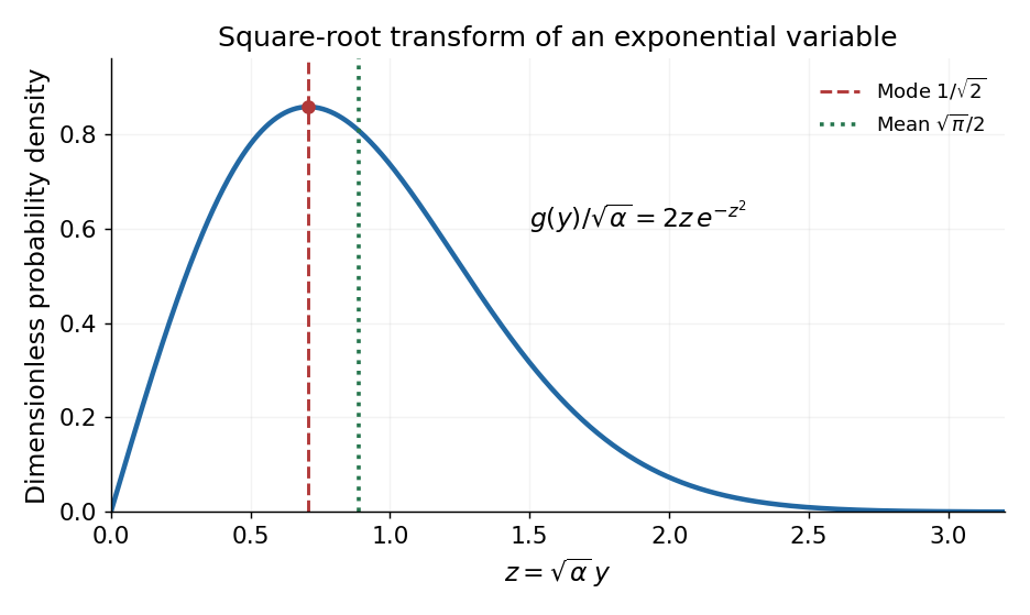
Normalize the probability density function on $x\ge 0$:For $y=\sqrt{x}\ge 0$, the change of variables is $x=y^2$, $dx=2ydy$. Conservation of probability gives the transformed probability density functionIt is a Rayleigh distribution with scale $\sigma =1/\sqrt{2\alpha }$. Its derivative is $g^{\prime }(y)=2\alpha e^{-\alpha y^2}(1-2\alpha y^2)$, so it rises from zero, has one maximum, and then decays:The expected value follows by putting $z=\sqrt{\alpha }y$:Here ${\int }_0^{\infty }{z}^2{e}^{-z^2}dz=\sqrt{\pi }/4$, obtained from the Gaussian integral by integration by parts. In particular $⟨\sqrt{x}⟩\ne \sqrt{⟨x⟩}$, and the mode changes under a nonlinear variable transformation because a density includes its Jacobian determinant.

For the binomial distribution, the binomial theorem givesDifferentiation of the probability generating function recovers the first expected value and second factorial moment:Since $X^2=X(X-1)+X$, the variance isThusThe formulas also hold for $n=0,1$ and the degenerate choices $p=0,1$, with derivatives read directly from the resulting polynomial.

For the discrete uniform distribution, each value has probability $1/n$. Using the given finite sums,Subtracting the square of the expected value gives the variance:Hence

Independence of random variables factors the joint probability mass function as $\mathbb{P}(X=x,Y=y)=\mathbb{P}(X=x)\mathbb{P}(Y=y)$. ThereforeWith finite expected values, these rearrangements are justified by absolute convergence: the analogous sum with absolute values equals $\mathbb{E}[|f(X)|]\mathbb{E}[|g(Y)|]<\infty$. Thus

On $0<x<2$, $2x-x^2=x(2-x)>0$. A valid probability density function must integrate to one, soThus $\alpha =3/4$, which is positive and ensures nonnegativity. Its expected value isThereforeThe probability density function is symmetric around $1$, providing a second check on the expected value.

Differentiate the probability generating function to obtainThe first derivative is the expected value, and the second gives the factorial moment $\mathbb{E}[X(X-1)]$. HenceIn particular, $\mathbb{E}[X^2]=q(2-p)/p^2$.

Put $S=X+Y$. Given $X$, its conditional expected value is $3X/2$ and its conditional variance is $X/4$, since $X$ is then fixed. The law of total expectation and law of total variance giveThe two scores are dependent: the law of total covariance gives $\mathrm{Cov}(X,Y)=\mathrm{Cov}(X,X/2)=q/(2p^2)$. Adding their two variances without that covariance term would give an incorrect total.