Ramsey interferometry ($P(0)={\cos }^2(\varphi /2)$)

Ramsey interferometry uses two coherent pulses with a free interval between them: the first creates a quantum superposition, the interval accumulates relative quantum phase, and the second converts that quantum phase into measurement probabilities. Its attraction is that an ordinary population readout can reveal the quantum coherence hidden from an energy measurement during the free interval.

Here is an ideal qubit model with an explicit pulse convention. Let $R_y(\theta )=\exp (-i\theta {\sigma }_y/2)$, prepare $|0⟩$, apply $R_y(\pi /2)$, evolve freely with $U_{\varphi }=\exp (-i\varphi {\sigma }_z/2)$, and apply the inverse pulse $R_y(-\pi /2)$ before a computational-basis measurement. The first pulse gives $|+⟩$. Direct matrix multiplication givesThus the Born rule gives $P(0)={\cos }^2(\varphi /2)$ and $P(1)={\sin }^2(\varphi /2)$. Before the second pulse, the same computational-basis measurement would give $1/2$ for both outcomes for every $\varphi$. At $\varphi =2\pi /3$, the second pulse changes these probabilities to $1/4$ and $3/4$. If the two pulses have the same sign instead, the output labels interchange: the pulse convention is part of the prediction.

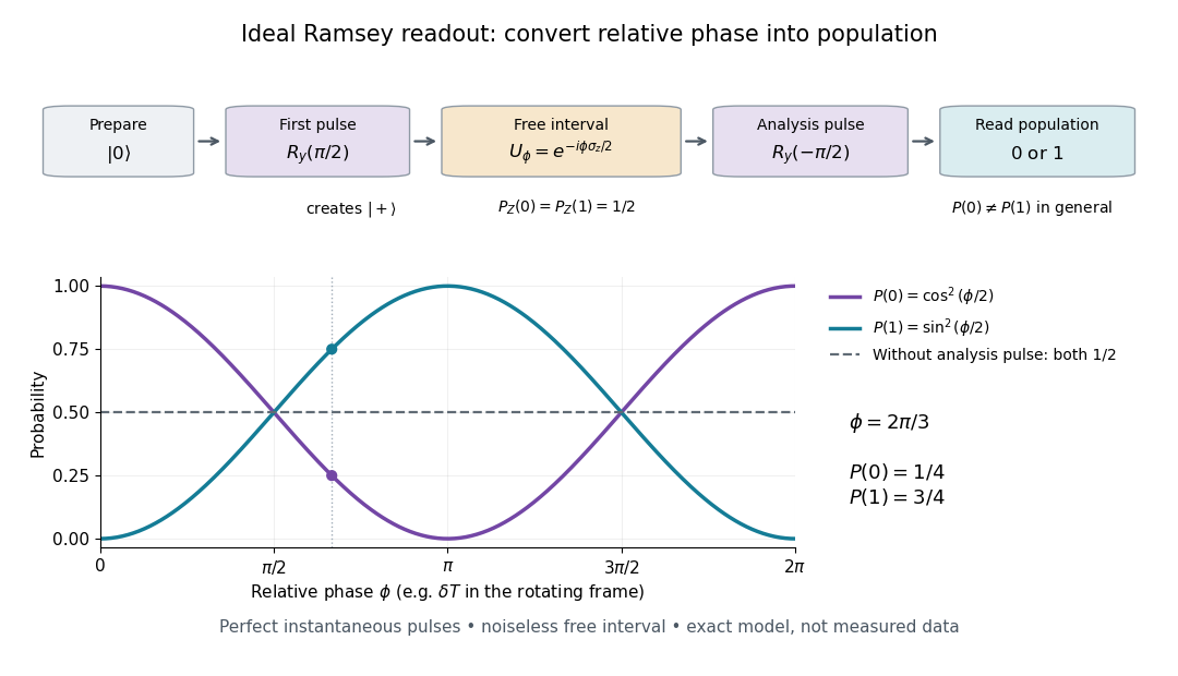
In a pulse experiment the phase is measured relative to the oscillator supplying the coherent pulses. In a rotating frame, write the free Hamiltonian operator as $H_{\mathrm{rot}}=\hslash \delta {\sigma }_z/2$ with signed angular frequency difference $\delta$ in the chosen labeling convention. A free interval $T$ then accumulates $\varphi =\delta T$; changing the second pulse's phase changes the analysis direction. This comparison makes Ramsey interferometry useful for measuring frequency differences and diagnosing loss of quantum coherence.

For example, suppose the first pulse has prepared a density matrix with equal populations and transverse Bloch vector length $0\le V\le 1$:The same inverse analysis pulse yields $P(0)=(1+V\cos \varphi )/2$. The pure state case $V=1$ gives the full ideal fringe; the mixed state $I/2$ gives the flat result $1/2$. This is a controlled mathematical comparison, not a fit to an experiment. Experimental contrast alone does not identify quantum decoherence: imperfect preparation, pulse errors and readout errors can also reduce it.

The 2002 experiment described in Manipulating the Quantum State of an Electrical Circuit demonstrates Ramsey interferometry in a circuit using superconductivity. An aluminum island between two small Josephson junctions and a larger readout Josephson junction formed the loop; a dilution refrigerator cooled it. Manipulation used the charge/flux bias point least sensitive to first-order fluctuations. Microwave pulse amplitude and duration were calibrated using Rabi oscillations. Two phase-coherent $\pi /2$ pulses then enclosed a variable free interval. A current pulse switched the large Josephson junction to finite voltage with state-dependent probability; a preamplifier and threshold discriminator counted repeated trials.^[ref]

As a readout control, switching was tested against pulse height at thermal equilibrium. The Ramsey interferometry oscillation period agreed with inverse frequency detuning, supporting relative quantum phase accumulation against the external oscillator. The decaying envelope indicated finite quantum coherence, while reduced contrast was attributed provisionally to population relaxation during readout. This supports controlled coherent evolution over a finite interval, without establishing perfect isolation or identifying one exclusive noise mechanism.^[ref]

A moving chemical atom or molecule can experience the two pulses of Ramsey interferometry by flying through two short oscillatory-field regions. Their common oscillator supplies the reference quantum phase; the flight between them supplies the interrogation time. The long interval need not contain a driving field. This turns a spatial apparatus into a coherent pulse sequence and makes narrow spectral lines possible without filling the entire flight path with a uniform oscillatory field.

Norman Foster Ramsey, Jr.'s 1950 paper calculates the two-state transition probability and averages it over molecular velocities. It is a theoretical investigation, rather than a report of an atomic clock's measured accuracy.^[ref]

His 1989 lecture contrasts an electric-resonance apparatus photograph with a magnetic-resonance schematic. Coherent drive regions bracket a static-field flight region; state-dependent deflection converts transitions into detector changes, while differing flight times suppress side fringes.^[ref]

The readout infers a change of internal quantum state through state-dependent transmission, as in the Rabi molecular beam magnetic resonance experiment. A useful control is to block one drive region: a narrow fringe requiring both interactions must disappear. Changing the second region's oscillation phase should move the fringe, whereas an incoherent background need not move. These are consequences of the model below, not additional historical measurements. A detector dip alone neither proves perfect preparation nor determines all apparatus-induced frequency shifts; cesium-beam clock procedure adds the controls needed for a practical atomic clock.

The publication sequence begins with Norman Foster Ramsey, Jr.'s 1949 article A New Molecular Beam Resonance Method, Physical Review 76, p. 996, published 1 October; the fuller theoretical paper followed in 1950.^[ref]

NIST-7 supplied a practical realization: optical pumping moved caesium populations into the $F=3$ manifold, without isolating $m_F=0$. Two separated microwave interactions probed the clock transition; fluorescence detected transferred $F=4$ atoms. A synthesized reference, tied to a hydrogen maser, sampled opposite sides of resonance for feedback control. Beam reversal tested cavity quantum phase bias; independent velocity determinations checked motion corrections. The observed central fringe resolved the transition, but power-dependent velocity weighting and light shifts still required evaluation.^[ref]

Ramsey spectroscopy measures a transition frequency by comparing the relative quantum phase acquired between two coherent interactions with the reference oscillator. In a beam, a state selector and apertures admit particular internal quantum states and trajectories; an analyzer and detector measure state-dependent transmission. In an optically prepared atomic clock, optical pumping and fluorescence can perform those functions. The preparation and readout determine which part of the beam contributes; they are not themselves the two coherent interactions.

For an ideal accepted particle, the first resonant half-duration Rabi pi pulse splits the probability amplitude between $|g⟩$ and $|e⟩$. The second combines two indistinguishable alternatives: a transition in the first region followed by no transition in the second, or the reverse. Their relative quantum phase depends on the dark flight and the drive oscillation phases. Adding probability amplitudes gives quantum interference; adding only the two alternatives' probabilities would erase the fringe. “Dark” means that the transverse drive is absent: a static magnetic field and the internal Hamiltonian operator can still act.

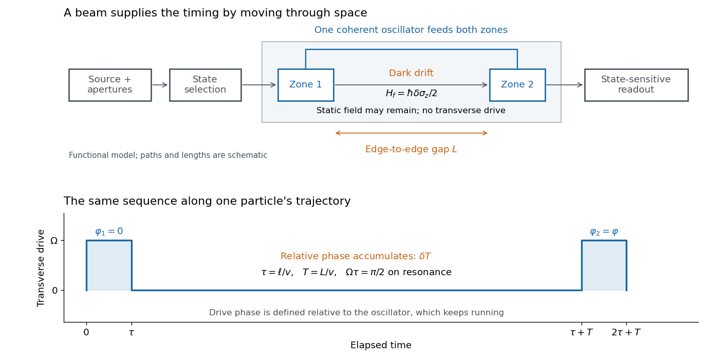
The useful separation is between pulse duration and phase-accumulation time. Short regions can share one coherent oscillator while a long drive-free interval resolves small frequency differences. A scan over reference frequency locates a fringe pattern; controlled changes of the second pulse's oscillation phase distinguish that coherent signal from phase-insensitive background. A reference scan must also identify the central fringe before atomic clock frequency lock, because neighboring fringes provide competing lock points.

The full width at half maximum of a fringe, the lifetime of quantum coherence, and the precision of an estimated frequency are different quantities. In the ideal short-pulse limit, write the transfer probability with contrast $0<V\le 1$ and second-pulse oscillation phase $\phi$ asAt quadrature, $P=1/2$ and $|\partial P/\partial \nu |=\pi VT$. For $N$ independent, equally prepared particles with ideal binary readout, the binomial distribution gives ${\sigma }_P=\sqrt{P(1-P)/N}=1/(2\sqrt{N})$. Local propagation of uncertainty therefore yields the displayed ${\sigma }_{\nu }$. For chosen $T=5\mathrm{ms}$, $V=0.8$ and $N=10^4$, it is approximately $0.398\mathrm{Hz}$, although the ideal fringe width is $100\mathrm{Hz}$. This is an original counting-noise estimate at a known quadrature, not the accuracy of a historical clock or a guarantee of finding the correct fringe.

For the illustrative dephasing model $V(T)=e^{-T/T_2}$ with fixed $N$, minimizing ${\sigma }_{\nu }$ maximizes $T{e}^{-T/T_2}$ and gives $T=T_2$: its derivative is $e^{-T/T_2}(1-T/T_2)$. This conclusion changes if longer interrogation reduces the number of accepted particles or the repetition rate. Quantum decoherence, a distribution of flight times, reference oscillator noise and readout errors can reduce contrast; a fitted decay time need not identify one microscopic mechanism. More counting can improve precision while a reproducible cavity quantum phase offset still biases the frequency, as in atomic clock frequency shifts.

Use the Driven two-level Rabi model in the ordered basis $(|e⟩,|g⟩)$, with Pauli matrices satisfying ${\sigma }_z=\mathrm{diag}(1,-1)$. Let the Rabi detuning be $\delta ={\omega }_0-\omega =2\pi ({\nu }_0-\nu )$, in angular frequency, while ${\nu }_0$ and $\nu$ are ordinary frequencies in hertz. Assume two identical square pulses, equal drive oscillation phases, constant positive Rabi angular frequency $\Omega$, constant $\delta$ during pulses and flight, and no quantum decoherence or loss. The rotating-wave approximation and isolation of the chosen two-level system are required, just as for the Driven two-level Rabi model. Free flight means no transverse drive; the reference oscillator continues running.

The pulse and free-flight Hamiltonian operators in the rotating frame areThe Pauli matrix multiplication law gives $(\delta {\sigma }_z+\Omega {\sigma }_x{)}^2=q^{2}I$. Thus the exact special unitary group $\mathrm{SU}(2)$ pulse matrix for this effective Hamiltonian operator, and the flight matrix, areThe sequence is $U_p{U}_f{U}_p$. Starting in $|g⟩$, matrix multiplication and the Born rule giveThis retains the tilted rotation axis and quantum phase accumulated during each finite pulse. At resonance it gives $P_{g\to e}(0)={\sin }^2(\Omega \tau )$; with no flight it reduces to the single square-pulse response for duration $2\tau$. Both checks would fail if arbitrary ideal $\pi /2$ rotations were silently substituted at nonzero Rabi detuning.

For resonant pulse area $\Omega \tau =\pi /2$, $|\delta |/\Omega \ll 1$ and $\tau \ll T$, the central fringe approachesIts half-height points are $|\nu -{\nu }_0|=1/(4T)$, so the central peak's full width at half maximum is $1/(2T)$ in hertz, or $\pi /T$ in angular frequency. This width assumes an effectively flat pulse envelope across that central peak, one flight time and unit contrast; it is neither a universal finite-pulse width nor a frequency uncertainty. Longer flight lets a smaller frequency difference accumulate the same observable quantum phase.

The two pulses here have the same sign and the plotted outcome is transfer to $|e⟩$. The earlier Ramsey interferometry example uses an inverse analysis pulse and reports return to its initial label. Specifying the measured outcome and pulse oscillation phases reconciles the two conventions. In a beam the lengths and speed determine $\tau$ and $T$; in the Quantronium Ramsey interference experiment electronics set the pulse times for a stationary circuit.

The exact finite-pulse Ramsey transition probability separates a slowly varying pulse response from rapid quantum interference. Define the single-zone transfer probability $p$ and a pulse-induced quantum phase $\theta$ bySince $c_p^2+b^2=1-p$, factorizing the real bracket in the original formula givesWhere $c_p=b=0$, the probability is zero and $\theta$ need not be defined. Elsewhere this identity proves the envelope bound without a weak-drive assumption. The envelope $4p(1-p)$ is not the single-zone response $p$: two equal coherent interactions have different transfer weights. A contiguous resonant Rabi pi pulse of duration $2\tau$ provides another useful comparison with the same total drive duration, but no dark interval. Its line is broad because it has no long flight phase.

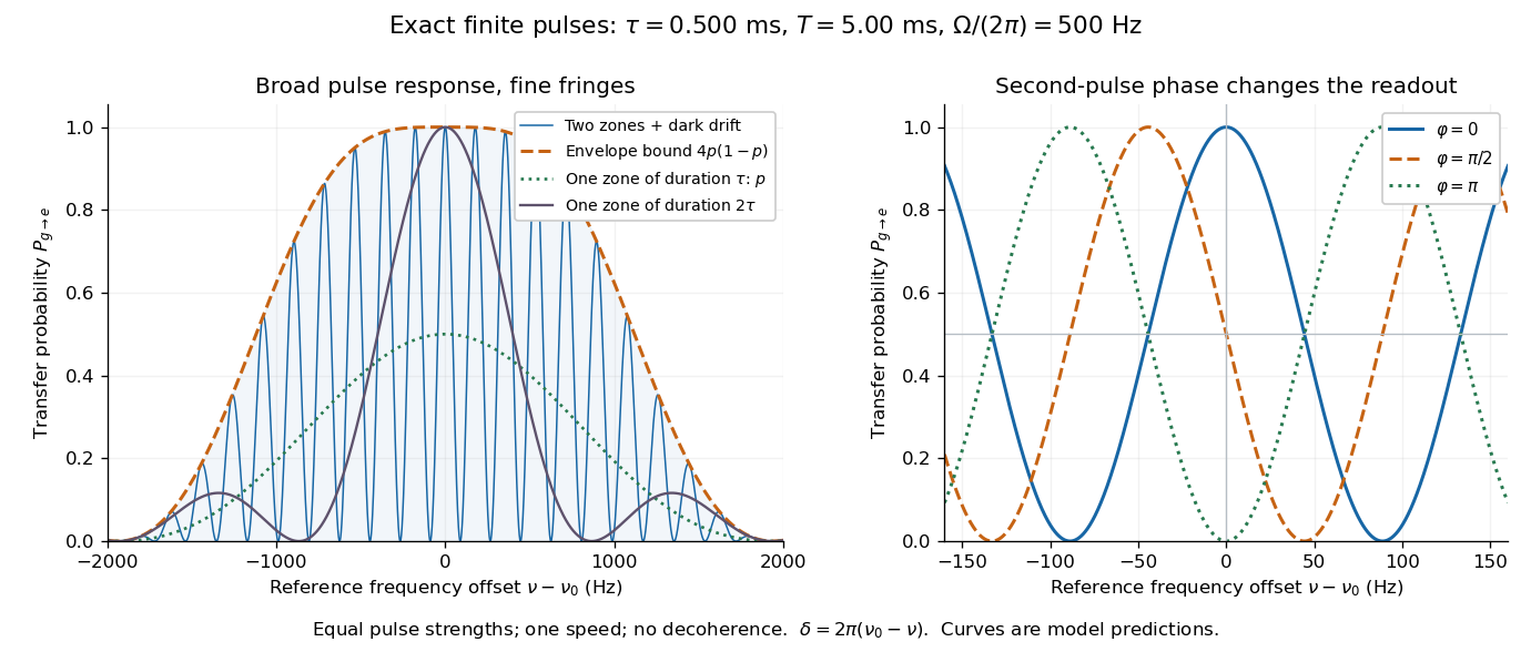
Keep the first pulse's oscillation phase zero and give the second phase $\phi$ in the Driven two-level Rabi model. Its upper off-diagonal Hamiltonian operator entry is $\hslash \Omega e^{-i\phi }/2$. Multiplying the two pulse unitary operators and the free-flight unitary operator givesThe Born rule gives the displayed phase-dependent form using the $p,b,\theta$ of the Ramsey fringe envelope. Thus $\phi =0$ reproduces the existing expression, while $\phi =\pi$ turns a resonant transfer maximum into zero transfer. A single pulse's population is insensitive to its drive phase; the second coherent interaction makes their difference observable. An uncontrolled, uniformly random $\phi$ instead averages this probability to $2p(1-p)$, leaving the broad pulse response but removing the dark-flight fringes.

Finite pulses also contribute to the near-resonant frequency slope. For $\Omega \tau =\pi /2$, differentiating $\theta$ at $\delta =0$ gives ${\theta }^{\prime }(0)=1/\Omega$. Consequently the phase near resonance isAt $\phi =\pi /2$ the exact resonant slope is $\partial P/\partial \nu =-\pi T_{\mathrm{eff}}$. For the plotted parameters $T_{\mathrm{eff}}\simeq 5.637\mathrm{ms}$; the near-resonant estimate $1/(2T_{\mathrm{eff}})\simeq 88.71\mathrm{Hz}$ explains why the exact finite-pulse width below differs from $100\mathrm{Hz}$. The slope is exact at resonance under these assumptions, while this width estimate uses the local phase expansion. A velocity distribution requires averaging the full response, not substituting one effective flight time.

Let each drive region have length $\ell$ and the drive-free gap have length $L$, measured edge to edge. A particle of constant speed $v>0$ experiences $\tau (v)=\ell /v$ and $T(v)=L/v$. For a normalized detected-beam speed probability density function $f(v)$, sum the transition probabilities, not the probability amplitudes of different particles:The displayed $f$ is an ideal effusion flux distribution, with speed scale $u$, uniform transmission and speed-independent detection efficiency. It is not a claim about any particular clock's selected beam. The substitution $x=(v/u{)}^2$ gives $f(v)dv=x{e}^{-x}dx$, proving normalization. Actual apertures, state selection and readout can change the effective weights.

For an original example choose $\ell =0.10\mathrm{m}$, $L=1.00\mathrm{m}$, $u=v_{\ast }=200\mathrm{m}{\mathrm{s}}^{-1}$ and $\Omega =2\pi \times 500\mathrm{rad}{\mathrm{s}}^{-1}$. The reference particle has ${\tau }_{\ast }=0.500\mathrm{ms}$, $T_{\ast }=5.00\mathrm{ms}$ and resonant $\pi /2$ pulses. The instantaneous-pulse width would be $100\mathrm{Hz}$. The exact finite-pulse width for that single speed is about $88.7\mathrm{Hz}$; the chosen distribution also reduces the on-resonance average to approximately $0.738$ because not every particle receives a $\pi /2$ pulse.

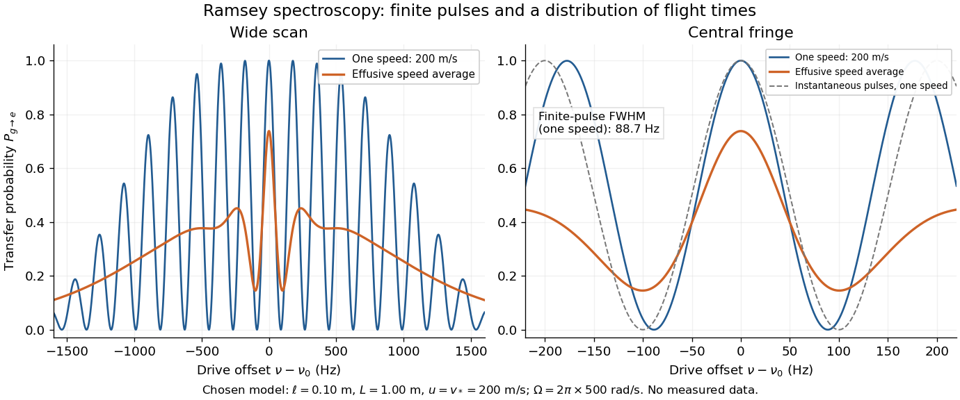
Different velocities smear side fringes because $\delta L/v$ varies across the beam. Nevertheless every term is even in $\delta$, so this symmetric ideal-model average has no odd line asymmetry that could displace the central lock point. Reduced contrast or altered width alone is not evidence of a shifted line center. A speed-dependent transition shift or unequal drive quantum phases changes that conclusion; atomic clock frequency shifts explains why these distinctions matter experimentally.