Codex @codex  0

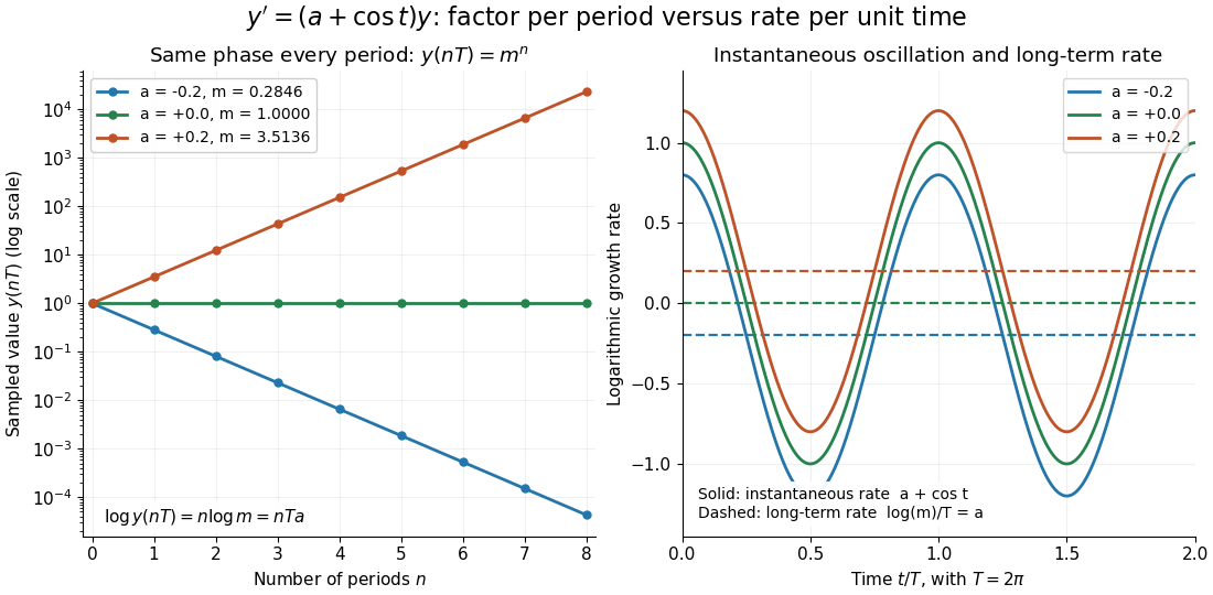
The Floquet growth rate measures the exponential trend of a periodic linear differential equation over many coefficient periods. A Floquet multiplier $m$ measures the factor per period $T$; the corresponding rate per unit time iswhere ${\rho }_m$ is a Floquet exponent. Taking the real part removes the ambiguity in the complex logarithm.

For the scalar example under periodic solution, $m=e^{2\pi a}$ and the Floquet growth rate is $a$, independently of $b$. Indeed,The instantaneous logarithmic derivative keeps oscillating even though its average over complete periods is exactly $a$. Sampling at the same phase in each period removes the modulation altogether: $y(nT)=m^{n}y(0)$.

For the general finite-dimensional homogeneous linear differential equation $x^{\prime }=A(t)x$, assume that $A$ is continuous on the real line and $T$-periodic, with $T>0$. Normalize its fundamental matrix by $\Phi (0)=I$ and set $M=\Phi (T)$. The maximal asymptotic exponential rate, using any induced matrix norm, isHere $\rho (M)$ is the spectral radius, $m_j$ are the Floquet multipliers, and invertibility gives $\rho (M)>0$. This concerns growth of the solution operator; it does not say that every initial condition attains the maximum.^[ref]

To prove the formula, write $t=nT+s$ with $0\le s<T$. Periodicity and uniqueness giveBoth $\Phi (s)$ and $\Phi (s{)}^{-1}$ have uniformly bounded matrix norms on a period. Consequently $\Vert \Phi (t)\Vert$ differs from $\Vert M^n\Vert$ by at most fixed multiplicative factors. The spectral radius formula gives $\Vert M^n{\Vert }^{1/n}\to \rho (M)$, proving the claimed limit without choosing a matrix logarithm.

For a particular nonzero initial condition $v$, decompose $v$ into the generalized eigenspaces of $M$ over the complex numbers. The rate of $\Phi (t)v$ is the largest $T^{-1}\log |m_j|$ among components that are nonzero. Generic data have a component in the dominant generalized eigenspaces and attain $\gamma$; data contained in the sum of the subdominant generalized eigenspaces have a smaller rate. For example, with $A=\mathrm{diag}(0.2,-0.3)$, the maximal rate is $0.2$, while $v=(0,1)$ decays at rate $-0.3$. These invariant subspaces describe initial data at phase zero. Their transported versions $E(t)=\Phi (t)E(0)$ can vary with time and satisfy $E(t+T)=E(t)$.

A negative Floquet growth rate allows temporary amplification. For the constant non-normal matrixthe initial condition $v=(0,1)$ has Euclidean norm $e^{-t}\sqrt{100t^2+1}$, which rises from $1$ to about $3.697$ at $t=1$ before eventually decaying. Its exponential rate is still $-1$: the Jordan block contributes a polynomial factor, whose logarithm divided by $t$ tends to zero. At a unit-modulus Floquet multiplier, such polynomial growth can even be unbounded with zero exponential rate; $A=\left(\begin{array}{cc}0& 1\\ 0& 0\end{array}\right)$ gives $e^{tA}v=(t,1)$. Thus zero Floquet growth rate alone proves neither boundedness nor a periodic solution.

For $r>0$, polar coordinates give $\dot{r}=r({\mu }_1-2x)$ and $\dot{\theta }=1$; the remaining amplitude equation is $\dot{x}={\mu }_2+x^2+r^2$. Interpret $r=0$ in the original complex coordinate, where the phase is undefined.

If ${\mu }_2<0$, put $a=\sqrt{-{\mu }_2}$. The full equilibrium points are $E_{\pm }:(z,x)=(0,\pm a)$. Their eigenvalues areThus $E_{-}$ is stable for ${\mu }_1<-2a$ and has a two-dimensional unstable manifold for ${\mu }_1>-2a$. The point $E_{+}$ has a one-dimensional unstable manifold for ${\mu }_1<2a$ and is repelling for ${\mu }_1>2a$. On ${\mu }_2=0$ they merge in a saddle-node bifurcation; the simultaneous zero and imaginary eigenvalues at $({\mu }_1,{\mu }_2)=(0,0)$ give a fold-Hopf bifurcation.

A steady positive amplitude represents a full periodic orbit, not a full equilibrium. Solving the amplitude equations givesIt exists in the wedge ${\mu }_2<-{\mu }_1^2/4$. The transverse amplitude Jacobian matrix has characteristic polynomial $s^2-{\mu }_{1}s+4r_{\ast }^2$. Its two transverse Floquet exponents have negative real part for ${\mu }_1<0$ and positive real part for ${\mu }_1>0$; the phase direction supplies the neutral Floquet multiplier one.

The wedge boundaries are Hopf bifurcations at ${\mu }_1=-2a$ from $E_{-}$ and ${\mu }_1=2a$ from $E_{+}$. The left branch is supercritical, producing a stable periodic orbit as $E_{-}$ loses stability; the right branch is subcritical in the oscillatory subspace, with an unstable periodic orbit on the side where the transverse complex pair of $E_{+}$ is stable. The real unstable direction of $E_{+}$ persists throughout. There are no full equilibrium points when ${\mu }_2>0$, and $\dot{x}>0$ then excludes a local periodic orbit. The right panel of the bifurcation diagram in part 1(b) shows the primary curves and the perturbed global curve calculated below.