A history function of a delay differential equation supplies the past interval needed to start a retarded delay differential equation. A single initial condition generally leaves earlier delayed values unspecified.[ref]
Delay-differential equations by Skip Thompson. Skip Thompson, Delay-differential equations, Initial History Function: prescribing the solution before the starting time
For a continuous function history, the natural state at time is the entire segmentIt belongs to the function space , an infinite-dimensional vector space: the functions are linearly independent. Shifting forward retains the part of the past that the equation can still read. Thus even one scalar unknown can require a state in an infinite-dimensional vector space.
The insufficiency of one value is visible without any approximation. Consider with the two history functions of a delay differential equationBoth give , yet on the first step the respective derivatives are and . Direct integration givesIn particular while . On the next step,At they are and , a gap of . These different futures reflect different prescribed histories; each fully specified problem has a unique solution of a differential equation. More strongly, for with , observing the entire first-step derivative recovers every history value through for , using the right derivative at . The future can depend on the whole function, rather than a finite list of its samples.
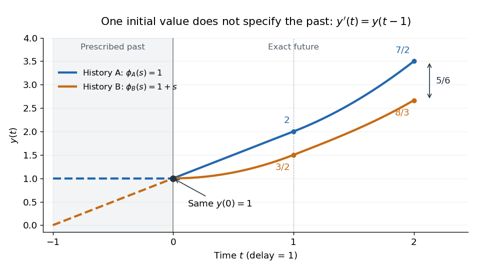
Equal initial values and different histories give different futures
. Two exact solutions of a differential equation for . Dashed curves are the prescribed history functions of a delay differential equation; solid curves are their exact continuations. Both pass through . The endpoint values and come from the displayed polynomials, with no numerical time stepping. Details.
Articles by others on the same topic
There are currently no matching articles.