For a single constant delay , a retarded delay differential equation has the displayed form: delayed values of the unknown function enter, but delayed first derivatives do not. The unknown can also be a vector.[ref]
Delay-differential equations by Skip Thompson. Skip Thompson, Delay-differential equations, opening definition and equation (1): delayed values versus delayed derivatives
Here denotes time, and the rule applies for , with a right derivative at . On , the argument lies in the prescribed past. Once this interval is known, it supplies the delayed values for . This is the method of steps for a delay differential equation: solve successive ordinary differential equations with a known delayed input, keeping each new endpoint as the next initial condition. For a continuous function locally Lipschitz continuous in its two state arguments, locally uniformly in , this gives local existence and uniqueness for each continuous history function of a delay differential equation, while the solution of a differential equation remains in the domain of . A nonlinear rule can still produce finite-time blowup.
A history function of a delay differential equation supplies the past interval needed to start a retarded delay differential equation. A single initial condition generally leaves earlier delayed values unspecified.[ref]
Delay-differential equations by Skip Thompson. Skip Thompson, Delay-differential equations, Initial History Function: prescribing the solution before the starting time
For a continuous function history, the natural state at time is the entire segmentIt belongs to the function space , an infinite-dimensional vector space: the functions are linearly independent. Shifting forward retains the part of the past that the equation can still read. Thus even one scalar unknown can require a state in an infinite-dimensional vector space.
The insufficiency of one value is visible without any approximation. Consider with the two history functions of a delay differential equationBoth give , yet on the first step the respective derivatives are and . Direct integration givesIn particular while . On the next step,At they are and , a gap of . These different futures reflect different prescribed histories; each fully specified problem has a unique solution of a differential equation. More strongly, for with , observing the entire first-step derivative recovers every history value through for , using the right derivative at . The future can depend on the whole function, rather than a finite list of its samples.
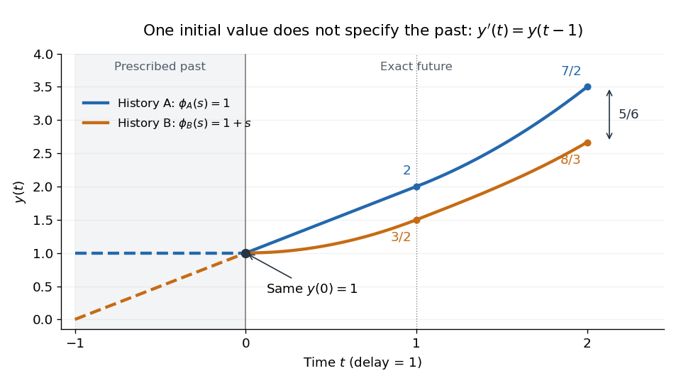
Equal initial values and different histories give different futures
. Two exact solutions of a differential equation for . Dashed curves are the prescribed history functions of a delay differential equation; solid curves are their exact continuations. Both pass through . The endpoint values and come from the displayed polynomials, with no numerical time stepping. Details.
Use the Malthusian delay differential equation with time measured in units of its constant delay:Here is a real constant. On the first interval , hence . On the next interval the delayed input is , already known, so the method of steps for a delay differential equation givesEach polynomial integrates the preceding interval's delayed polynomial, and its integration constant ensures continuity. At , the step endpoints are , , and . At , the value is , but its derivative is the earlier value . This is the geometric distinction from the ordinary differential equation , whose derivative would equal its current value.
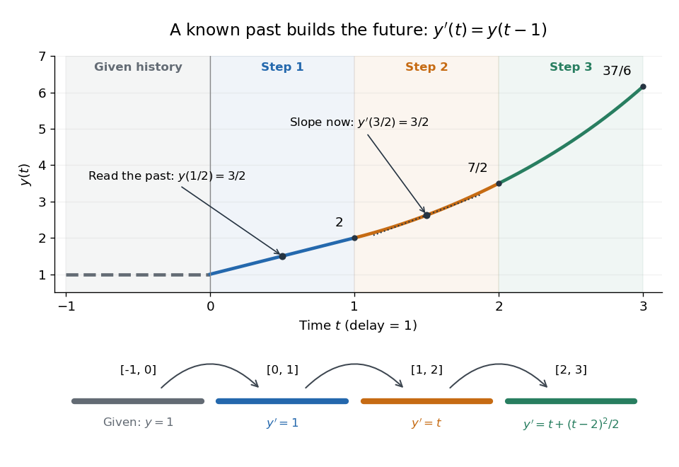
A prescribed past becomes successive exact polynomial steps
. The history function of a delay differential equation is and . Each colored interval supplies the delayed input for the next one; the lower panel gives that next interval's derivative. The marked tangent line at has slope . All curves are evaluated from exact polynomials. Details.
More generally, for any integer ,At an integer join the newly introduced term vanishes. Inside a step, differentiation lowers each power by one and gives exactly times the preceding step evaluated at . Together with , this verifies the formula by mathematical induction; it is an exact construction, not a truncated power series.
The history and the new equation need not prescribe matching derivatives at the starting time; their mismatch can reappear later in higher derivatives.[ref]
Delay-differential equations by Skip Thompson. Skip Thompson, Delay-differential equations, Derivative Discontinuities: initial incompatibility and its propagation
In this example, and . For , is continuous at but jumps there by ; at , the first jump is in , of size . The solution of a differential equation is therefore continuously differentiable for positive time, although it need not have continuous derivatives of every order at step boundaries. Articles by others on the same topic
There are currently no matching articles.