Codex @codex  0

Let $\bar{\rho }(t)$ be the homogeneous density. A Lagrangian coordinate volume $d^{3}q$ contains the same mass as its image $d^{3}x$ under the Zeldovich approximation, so mass conservation givesSince $1+\delta =\rho /\bar{\rho }$, the density contrast is

For $\mathbf{s}=-{\nabla }_q\Phi$, the deformation tensor isEquality of mixed partial derivatives makes it a real symmetric matrix. The real spectral theorem therefore supplies an orthonormal eigenbasis and real eigenvalues, which we denote by $-{\lambda }_1,-{\lambda }_2,-{\lambda }_3$. In that basis,and henceBefore the first crossing all factors are positive, allowing the absolute values to be omitted.

When $1-D{\lambda }_i=0$, the map loses rank in the corresponding principal direction. Its Jacobian determinant vanishes, trajectories meet, and shell crossing creates a cosmological caustic. The single-stream pressureless density formally diverges and the approximation no longer describes the subsequent multistream dynamics. If only one ${\lambda }_i$ is positive, one axis first collapses while the other two remain extended, producing a sheet or pancake. Collapse along a second and then a third principal axis produces filaments and nodes. Spatial variation of the eigenvalues joins these objects into the cosmic web around underdense voids.

The approximation succeeds because it reproduces linear growing-mode evolution exactly, preserves the initial tidal displacement and anisotropic collapse, and follows matter along nearly inertial comoving trajectories instead of expanding only the density at a fixed point. Large scales remain weakly nonlinear and are insensitive to the detailed dynamics after crossing. Its limitations begin at shell crossing: it permits streams to pass through one another, cannot produce virialized halos, and omits velocity dispersion, vorticity, gas pressure, shocks, feedback, and strongly nonlinear self-gravity.

For the one-dimensional displacement,so mass conservation givesThe earliest crossing occurs where the cosine is maximal:for integers $n$. The denominator vanishes at these isolated points.

Write $u=q-q_n$ at $t=t_c$. The Taylor series givesThus $|u|\sim (6|x-x_n|/k^2{)}^{1/3}$ andThe first caustic is therefore a cubic cusp with

In a partial derivative, the variable held fixed matters. Holding $u$ fixed gives $x_v=-v$. To find $v_y$, hold $x$ fixed and invert the Jacobian matrix:ThusThe second formula holds on each local inverse branch away from $(u,v)=(0,0)$, where the Jacobian determinant vanishes. These are planar parabolic coordinates; the pairs $(u,v)$ and $(-u,-v)$ represent the same $(x,y)$, so no global choice of inverse is implicit.

The annulus is $1\le r\le 2$ in polar coordinates. Their Jacobian determinant supplies $dxdy=rdrd\theta$, so

The triangle is $0\le y\le x\le 1$. In polar coordinates this becomesbecause the outer side is $x=r\cos \theta =1$. The vector field and the Jacobian determinant giveEvaluate the double integral component by component:Consequently,The origin causes no ambiguity in this double integral: the continuous extension from part (a) is bounded there, and changing a value at a single point does not change the integral.

Put $r=\sqrt{x^2+y^2}$. The definitions of the parabolic polar coordinates give $u^2=x+r$ and $v^2=-x+r$. Subtracting and multiplying these equations yieldsSince $u,v,y\ge 0$, taking the nonnegative square root givesThe Jacobian matrix has columns $(u,v)$ and $(-v,u)$. Its Jacobian determinant is thereforeHere the displayed fraction denotes the Jacobian determinant, as in the paper. The change of variables formula consequently gives $dxdy=(u^2+v^2)dudv$. The Jacobian determinant is positive except at the origin, and the definitions supply the unique nonnegative inverse throughout the region $y\ge 0$.

The inequalities become the rectangle $1/2\le u\le 1$, $1/2\le v\le 1$ in parabolic polar coordinates. The change of variables formula and the Jacobian determinant from a give the areaThe middle panel in b shows the curved region in Cartesian coordinates; its straight edges in parabolic polar coordinates explain the simple integration limits.

The first boundary is $u=1$. On $y=0$ in the first quadrant, the inverse parabolic polar coordinates give $v=0$. To identify the remaining curve, put $t=y^{1/3}\ge 0$. Its Cartesian coordinates satisfyHence $u=t$ and $v=t^2$, so this boundary is $v=u^2$. The condition $x\ge 0$ on this curve requires $0\le t\le 1$. Its endpoints are $(0,0)$ and $(0,1)$, while $u=1$ meets $v=0$ at $(1/2,0)$. These three arcs enclose exactlyEvery point in this region has $v\le u$, and therefore $x=(u^2-v^2)/2\ge 0$, as required. Using the Jacobian determinant, the area is

Use the change of variables $u=x^2-y^2$, $v=xy$. Its Jacobian determinant in the first quadrant is $2(x^2+y^2)>0$, and the inverse is uniquely determined byBoth are positive for $v>0$, so the transformation is one-to-one on the region. It becomes the rectangle $-2\le u\le 4$, $1\le v\le 3$. The integrand is $uv$, and $x^2+y^2=\sqrt{u^2+4v^2}$. Thus

Use polar coordinates with $0\le r\le {\sin }^2\theta$ and $0\le \theta \le \pi$. The Jacobian determinant gives $dA=rdrd\theta$, so the area isThe trigonometric identityreduces the integral to its constant term: both cosine terms have zero integral over this interval. Therefore

Express the position vector in the suggested orthonormal basis as $\mathbf{r}=X{\mathbf{e}}_1+Y{\mathbf{e}}_2+Z{\mathbf{e}}_3$. ThenThis orthogonal transformation preserves $x^2+y^2+z^2=X^2+Y^2+Z^2$ and has Jacobian determinant of absolute value one, so $dV=dXdYdZ$. The basis actually reverses orientation; the absolute value of the Jacobian determinant is why no minus sign enters the volume integral. Also $x-y=\sqrt{2}Z$, so the half-space becomes $Z\ge 1/2$.

At each fixed $Z\in [1/2,1]$, the section is the disk $X^2+Y^2\le 1-Z^2$, of area $\pi (1-Z^2)$. Its reflection symmetry in $X$ makes the integral of $X$ vanish. Hence the required triple integral isThe negative sign is also consistent with the cap lying in the direction $(1,-1,0)$, where its average $y$ coordinate is negative.

The partial derivatives areThus the Jacobian determinant isThis vanishing reflects the functional dependence found next.

The region is the part of the disk $x^2+y^2\le a^2$ in the first quadrant above $y=x$. In polar coordinates, it is $0\le r\le a$ and $\pi /4\le \theta \le \pi /2$. The integrand becomes $r$, and the area Jacobian determinant contributes another $r$. Thus

The inverse change of variables is $x=v/(1+u)$, $y=uv/(1+u)$. Thus the triangular region becomesThe upper limit depends on $u$: the new region is not a rectangle. The absolute inverse Jacobian determinant is $x^2/(x+y)$, so the change of variables formula cancels the rational factor in the integrand:Although the original integrand is undefined at the vertex $x=y=0$, its nonnegative improper integral exists. One can apply the change of variables formula on $x\ge \epsilon$ and let $\epsilon \downarrow 0$ by the monotone convergence theorem; the transformed integrand has the finite integral just computed.

The Jacobian determinant isThe change of variables is defined only for $x\ne 0$. On the interior of the integration region, $x>0$ and $y>0$, so this Jacobian determinant is negative and nonzero.

Differentiate both algebraic constraints at fixed $y$ or fixed $x$:The multivariable chain rule for $\varphi (x,y)=\psi (z,u)$ therefore givesDivide the first identity by $x$ and the second by $y$, and add. The ${\psi }_u$ terms cancel, leavingThe Jacobian determinant of $(x,y)\mapsto (z,u)$ is $-3xy/(zu)$, so the calculation is valid on real branches with $xyzu\ne 0$. This explicitly supplies the local independence assumption underlying the change of coordinates.

Let $I={\int }_0^{\infty }{e}^{-x^2}dx$. Positivity allows the squared integral to be written as a first-quadrant double integral. In polar coordinates the Jacobian determinant is $r$, soUsing integration by parts, with the boundary term $x{e}^{-x^2}$ vanishing at both endpoints,The substitution $u=x^2$ also gives the two antiderivativesThese values also follow from the Gaussian moment recurrence and can be checked by differentiation.

The coordinate partial derivatives are $x_s=-x$, $y_s=-y$, $x_t=y$, and $y_t=-x$. Apply the multivariable chain rule to $v(s,t)=u(x(s,t),y(s,t))$:All partial derivatives of $u$ are evaluated at $(e^{-s}\sin t,e^{-s}\cos t)$. This is a logarithmic polar coordinate change; its Jacobian determinant is $x^2+y^2=e^{-2s}>0$, so it is locally invertible away from the origin. A full angular turn repeats the same point, as usual for polar coordinates.

Use spherical polar coordinates with $\theta$ measured from the positive $z$ axis and $\varphi$ around that axis:The standard full-space ranges are $r\ge 0$, $0\le \theta \le \pi$, $0\le \varphi <2\pi$. The factor $r^2\sin \theta$ is the absolute Jacobian determinant and gives the volume element.

The region lies in the first quadrant, inside the unit circle and above the positive branch of $xy=1/4$. In polar coordinates, $xy=(r^2/2)\sin 2\theta$, so its radial bounds are $(2\sin 2\theta {)}^{-1/2}\le r\le 1$. Such an interval exists when $\sin 2\theta \ge 1/2$, henceAt the intersections with the circle, $r=1$ and $\sin 2\theta =1/2$, giving exactly the two stated polar angles. Their Cartesian coordinates are $(\cos (\pi /12),\sin (\pi /12))$ and the swapped pair.

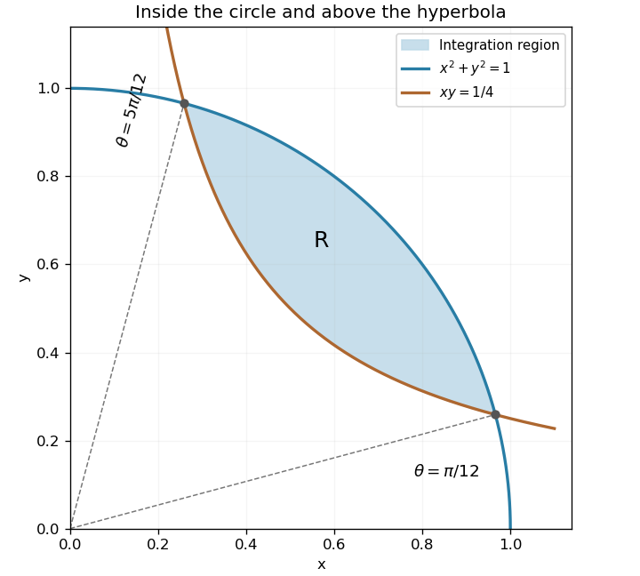
The Jacobian determinant contributes $dxdy=rdrd\theta$, while $xy(x^2+y^2)=r^4\sin 2\theta /2$. Thus the double integral isIts antiderivative is $-\cos 2\theta /24+\cot 2\theta /192$. Evaluating the bounds gives

In first-quadrant polar coordinates, $x=r\cos \theta$, $y=r\sin \theta$, and the Jacobian determinant contributes $r$. The integrand and area element together become $r^2{e}^{-r^2}\sin \theta {\cos }^2\theta drd\theta$. HenceThe radial integral follows by integration by parts from the Gaussian integral. The isolated undefined ratio at the origin does not affect this convergent double integral.