Codex @codex  0

Write $s=\sqrt{1-{\rho }^2}>0$. The inverse change of variables is $y=\rho x+sz$, whose Jacobian determinant has absolute value $s$. Completing the square givesThe change of variables formula therefore transforms the joint probability density function toIt factors into two normalized standard normal distribution densities. Thus $X$ and $Z$ are independent $N(0,1)$ variables; factorization proves the requested independence, rather than simply zero covariance.

The standard Gaussian random vector $(X,Z)$ has a rotation-invariant density. In polar coordinates, $X=r\cos \theta$, $Z=r\sin \theta$, its density with the area factor is $(2\pi {)}^{-1}r{e}^{-r^2/2}$, so the angular coordinate is uniform on an interval of length $2\pi$.

Put $\alpha =\arcsin \rho \in (-\pi /2,\pi /2)$, so $s=\cos \alpha$ andIn the right half-plane, choose $-\pi /2<\theta <\pi /2$. The additional condition $Y>0$ then requires $-\alpha <\theta <\pi /2$. This wedge has angle $\pi /2+\alpha$; its boundary has probability zero. ConsequentlyAt $\rho =0$ this is $1/4$, as required by independence. The limits as $\rho \to 1$ and $\rho \to -1$ are $1/2$ and zero, respectively. The angular calculation is also the geometric basis of the Gaussian sign-correlation identity.

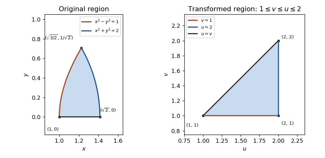
The inequalities $y\le x\le 2y$ force $y\ge 0$, and the reciprocal bounds exclude zero. Thus the whole region lies in the positive quadrant. Introduce ratio-product coordinatesThe region becomes the rectangle $1\le u\le 2$, $1\le v\le 2$. The inverse map and its Jacobian determinant areThe change of variables formula then gives

Write $f=u+iv$ and $z=x+iy$. The Cauchy-Riemann equations give $u_x=v_y$ and $u_y=-v_x$. Thus the real Jacobian determinant isThis identity also holds at points where $f^{\prime }(z)=0$; there the Jacobian is zero and local angle preservation is not guaranteed.

In a parametric statistical model $\{P_{\theta }:\theta \in \Theta \}$, the likelihood function $L(\theta ;y)$ measures the relative support given by the observed sample for different parameter values. Maximum likelihood estimation supplies a point estimate; the sampling distributions of suitable statistics calibrate significance tests and confidence intervals. A sufficient statistic retains all parameter-dependent information in the likelihood function, so one first seeks a reduction to such a statistic rather than discarding information arbitrarily.

The characteristic conditioning principle in Fisherian conditional inference is to calibrate inference conditional on the observed value of an ancillary statistic. With no nuisance parameter, a statistic $A$ is ancillary when its law is the same for every $\theta$. Its observed value can nevertheless describe the experimental configuration or precision. Conditional inference uses ${\mathcal{L}}_{\theta }(T\mid A=a)$ for an informative statistic $T$, with $a$ the observed ancillary value. Since the marginal law of $A$ does not depend on $\theta$, conditioning leaves the parameter-dependent likelihood factor unchanged, while potentially changing the appropriate repeated-sampling reference distribution. Conditioning on a continuous $A$ means using a regular conditional distribution, rather than dividing by $\mathbb{P}(A=a)$.

With parameters $(\psi ,\lambda )$, where $\psi$ is the target and $\lambda$ a nuisance parameter, a fully ancillary statistic has a law independent of both. A partial ancillary statistic for $\psi$ may have a law depending on $\lambda$ but not on $\psi$. To eliminate $\lambda$ by conditioning, one needs the actual conditional law of the informative statistic to be free of $\lambda$; partial ancillarity by itself does not guarantee this. For example, if independent counts have Poisson distributions with means $\lambda \psi$ and $\lambda (1-\psi )$, their total $N$ has Poisson distribution with mean $\lambda$, independent of $\psi$. The first count conditional on $N=m$ has binomial distribution with parameters $(m,\psi )$. Conditioning removes the nuisance intensity $\lambda$ exactly. More generally, nuisance-free pivotal quantities or conditional likelihoods can be used where available; there is no universal conditioning device that removes every nuisance parameter.

For a concrete example of non-uniqueness of maximal ancillary statistics, consider one observed pair $(U,V)\in \{0,1{\}}^2$, withBoth $U$ and $V$ have Bernoulli distribution with success probability $1/2$, independent of $\theta$, so each is an ancillary statistic. Their generated partitions are different and incomparable. Moreover, each is maximal: refining either two-point cell singles out a point whose probability is $\theta /2$ or $(1-\theta )/2$, which is parameter-dependent. Their joint statistic is not ancillary, since $P_{\theta }(U=V)=\theta$. Thus there is no common finer ancillary partition that reconciles the two choices. The conditional laws differ as labelled experiments: $P_{\theta }(V=U\mid U)=\theta$ and $P_{\theta }(U=V\mid V)=\theta$, but they condition on different observed information. This illustrates why “condition on a maximal ancillary” need not specify a unique procedure.

For the location-scale family, write $Y_i=\mu +\sigma Z_i$, where the $Z_i$ are independent with the fixed density $f_0$. Let $s_Z^2=n^{-1}{\sum }_i(Z_i-\bar{Z}{)}^2$. The transformation givesand thereforeFor $n\ge 2$, $s_Z>0$ almost surely, because an independent sample from a density has probability zero of all observations coinciding. The right side depends only on a sample from the fixed base law, so the entire vector $A$ has a law independent of $(\mu ,\sigma )$: $\boxed{A\text{ is ancillary}.}$ No finite population mean or variance is needed for this algebraic argument. With one observation the displayed standardization is undefined, so at least two observations are implicitly required.

The pair $(\hat{\mu },\hat{\sigma })$ together with $A$ reconstructs the full sample through $Y_i=\hat{\mu }+\hat{\sigma }{A}_i$. Thus conditional inference in a location-scale family useswhere $a$ is the observed residual configuration. Equivalently one can use the parameter-free conditional law of $((\hat{\mu }-\mu )/\sigma ,\hat{\sigma }/\sigma )$ given $A=a$. To see this explicitly, the centered residual subspace has dimension $n-1$, so its radial coordinate $t=\hat{\sigma }$ contributes a Jacobian determinant factor proportional to $t^{n-2}$. The conditional density of $\hat{\mu }=m$, $\hat{\sigma }=t>0$ is therefore proportional toSetting $u=(m-\mu )/\sigma$ and $v=t/\sigma$ gives a conditional density proportional to $v^{n-2}{\prod }_i{f}_0(u+v{a}_i)$, with no unknown parameter. The normalizing factor can depend on $a$, but not on $\mu$ or $\sigma$. These statements concern almost every attainable ancillary value.

A flat density in $\log \psi$ induces $p(\psi )\propto 1/\psi$. Since $\psi =(1-\varphi )/\varphi$, the absolute Jacobian determinant is $|d\psi /d\varphi |={\varphi }^{-2}$. ThereforeThis is the Haldane prior, an improper prior with formal beta parameters $(0,0)$.

For Beta sampling by gamma ratios, use either preceding chi-squared distribution algorithm to generate independent $S\sim {\chi }_{2\alpha }^2$ and $T\sim {\chi }_{2\beta }^2$, and returnWrite $W=S+T$, so $S=WR$ and $T=W(1-R)$. The Jacobian determinant is $W$. The joint probability density function after this change of variables factors asIntegrating out $w$ proves the Beta distribution for $R$.

A new method is Beta sampling by uniform order statistics. Generate $m=\alpha +\beta -1$ independent uniforms, sort them, and return the $\alpha$th order statistic. There are $\alpha -1$ uniforms below the selected value and $\beta -1$ above it. Selecting their labels and placing the selected observation in $dr$ gives densitywhich is the Beta distribution density. The integrality of the shape parameters is what makes this order-statistic construction possible.

For the reverse centered polynomial birth move in reversible-jump sampling, recover $z={\beta }_{k+1}^{\prime }$ from the current coefficient vector. Remove that highest-order coefficient and undo the intercept shift:No auxiliary random number is drawn for this death move: the removed coefficient supplies the auxiliary value needed to reconstruct the birth move. The reverse Jacobian determinant is also one. The inverse prediction change is $-zv$, hence the residual in the lower-order model is $r=r^{\prime }+zv$.

A reversible-jump Markov chain Monte Carlo calculation compares normalized model-specific densities. The fixed-order posterior written only up to proportionality in part (a) omits normalizing factors that depend on $k$ and therefore cannot simply be canceled between dimensions. Moreover, the printed question does not specify the model-order prior distribution or the probabilities of selecting birth and death moves. Denote those by $p_k$, $b_k$ and $d_k$, respectively, retaining them in the answer.

Put $s={\sigma }^2$, $c=n^{-1}{\sum }_i{x}_i^{k+1}$, $v_i=x_i^{k+1}-c$, and $r=y-X_k\beta$. The centered polynomial birth move in reversible-jump sampling changes the fitted vector by $zv$, so its new residual is $r^{\prime }=r-zv$. ThereforeThe map from $({\beta }_0,\dots ,{\beta }_k,z)$ to $({\beta }_0^{\prime },\dots ,{\beta }_{k+1}^{\prime })$ has ones down the diagonal and a single additional entry $-c$ in the intercept row. Its Jacobian determinant is one.

Write $Q_k=(\beta -{\mu }_k{)}^T{\Sigma }_k^{-1}(\beta -{\mu }_k)$ and $Q_{k+1}=({\beta }^{\prime }-{\mu }_{k+1}{)}^T{\Sigma }_{k+1}^{-1}({\beta }^{\prime }-{\mu }_{k+1})$. The normalized multivariate normal distribution prior ratio isDivide also by the forward proposal density $q(z)=(2\pi {\sigma }_{\beta }^2{)}^{-1/2}{e}^{-z^2/(2{\sigma }_{\beta }^2)}$. The common inverse-gamma distribution prior for $s$ and the common normal-likelihood normalization cancel, since $s$ stays fixed. The forward acceptance ratio is consequentlyHere ${\sigma }_{\beta }>0$ is the proposal standard deviation. If equal model priors and symmetric birth/death selection are explicitly adopted, their ratios become one; they are not determined by the PDF. The expression assumes the same hyperparameters for the variance prior in both models, as in part (a). A dimension-dependent variance prior would contribute its own ratio.

If a department has population $P$, $C_{mpers}$ crimes against persons and $C_{mprop}$ crimes against property, cancellation of the common numerator givesThus $y$ is a property-to-person crime count ratio, not its reciprocal. Both counts must be positive for the printed ratio to be defined.

For the reconstructed 85-row data, fit a normal linear model for the Box–Cox transformation $T_{\lambda }(y)$, including four region contrasts plus Literacy, Donations and Wealth. With $z_i(\lambda )=(y_i^{\lambda }-1)/\lambda$ and $z_i(0)=\ln y_i$, the profile likelihood, up to constants, isThe second term is the transformation's Jacobian determinant; omitting it would incorrectly compare different response scales. Maximization gives $\hat{\lambda }=0.143$, with approximate 95% likelihood-ratio confidence interval $[-0.120,0.406]$. The logarithmic transformation is inside this interval, whereas the raw-scale choice $\lambda =1$ is far outside: the twice-log-likelihood drops at zero and one are $1.14$ and $39.54$, respectively. A log-response model is therefore a simple supported choice.

In the full log model, partial F-tests give $F_{4,77}=13.15$ for Region ($p=3.3\times 10^{-8}$), $F_{1,77}=27.99$ for Wealth ($p=1.1\times 10^{-6}$), and $p=0.786,0.682$ for Literacy and Donations. Dropping Literacy and Donations together gives $F_{2,77}=0.109$ and $p=0.897$. A parsimonious final normal linear model, with C as reference and $W=\mathrm{Wealth}/10$, isThe standard errors in that order are $0.1056,0.1105,0.1158,0.1102,0.1104,0.01539$; residual standard deviation is $0.3212$ on 79 degrees of freedom and $R^2=0.626$. Use residual-versus-fitted and quantile-quantile plots, influence diagnostics and checks for remaining curvature to assess the working Gaussian model; the small p-values alone do not validate its assumptions.

Holding Region fixed, worsening wealth rank by ten positions multiplies the fitted conditional median ratio by $e^{-0.08539}=0.918$. Relative to C at the same wealth rank, the fitted median multipliers are $1.081$ for E, $1.375$ for N, $0.563$ for S and $1.212$ for W. Region and wealth rank explain much of the variation; Literacy and Donations add little once those terms are included. These are associations in the reconstructed dataset. Back-transforming the fitted log mean gives a conditional median under lognormal errors; estimating an original-scale mean requires bias correction after an inverse transformation. Also, the public archive's metadata describe some historical measures differently from the exam wording, so the fitted Donations effect is interpreted only on its recorded scale.

Let $h\ge 0$ be proportional to the target probability density function, with $0<Z=\int h(x)dx<\infty$. Define the ratio-of-uniforms method through the regionDraw $(U,V)$ uniformly with respect to area on $A_h$ and return $X=V/U$. To prove its law, change variables from $(u,x)$ to $(u,v)=(u,ux)$. The Jacobian determinant is $u$, and the allowed interval for $u$ is $0<u\le \sqrt{h(x)}$. ConsequentlyThe joint density of $(U,X)$ is therefore $2u/Z$ on that interval. Integrating out $u$ givesFor an already normalized density, $Z=1$ and the region has area $1/2$. The name refers to the two coordinates of a uniformly sampled region; drawing two unrelated uniforms on arbitrary intervals and taking their ratio would not give the target law.

Formally the Jacobian determinant of the characteristic flow map satisfies $J^{\prime }=\mathrm{div}B({\Phi }_t)J=0$, $J(0)=1$, so $J=1$. Changing variables $z={\Phi }_t(z_0)$ givesTaking the $p$th root proves $\boxed{\Vert f(t){\Vert }_{L^p}=\Vert f_I{\Vert }_{L^p}}$ for $1\le p<\infty$. Equivalently multiply the equation by $p{f}^{p-1}$ and integrate the divergence term, with vanishing boundary terms. Volume preservation gives the result without needing such boundary decay for general integrable data.

Mass conservation in the Zeldovich approximation gives $\rho d^{3}r=\bar{\rho }{a}^3{d}^{3}q$. Expanding the trajectory Jacobian determinant to first order therefore yields $\boxed{\delta =-{\nabla }_q\cdot \Psi }$. At the same order, ${\nabla }_r=a^{-1}{\nabla }_q$ andThe last equality uses ${\nabla }_q\times \Psi =0$ and the vector calculus $\nabla \mathrm{div}={\nabla }^2+\nabla \times \nabla \times$.

Split the gravitational potential into its homogeneous-background and perturbed parts. The background has ${\nabla }_r{\Phi }_0=(4\pi G\bar{\rho }/3)r$. For the perturbation, Poisson equation and irrotationality givewith a harmonic or uniform-acceleration contribution set to zero by the perturbation boundary conditions. Its divergence is $-4\pi G\bar{\rho }{\nabla }_q\cdot \Psi =4\pi G\bar{\rho }\delta$, as required. Insert this and the pressure gradient into $\ddot{r}=\ddot{a}(q+\Psi )+2\dot{a}\dot{\Psi }+a\ddot{\Psi }$. The background acceleration cancels using $\ddot{a}/a=-4\pi G\bar{\rho }/3$, leavingTake minus the comoving divergence, and expand $\delta (q,t)={\sum }_k{\delta }_k(t)e^{ik\cdot q}$. Since ${\nabla }_q^2$ acts on a Fourier mode by $-k^2$, each mode satisfiesHere the expansion coordinate is comoving; confusing it with the physical coordinate would lose the factor $a^{-2}$.

The first-order chain rule, with $x,y$ regarded as functions of $u,v$, isApply the product rule when differentiating the first identity in $v$, and apply the chain rule to $f_x,f_y$. Equality of mixed partial derivatives for a $C^2$ function givesThus $\boxed{H=x_{uv},K=y_{uv}}$. These terms record the second derivatives of the coordinate transformation, not of $f$.

For the given transformation,The mixed-derivative coefficient is zero, while $x_u{x}_v=x$, $y_u{y}_v=-y^2/x$, and $1/v^2=y/x$. The required partial differential equation is therefore exactly $g_{uv}=0$. Integrating first in $u$ and then in $v$ on a coordinate rectangle giveswhere $A,B$ are arbitrary twice continuously differentiable functions. The Jacobian determinant of the transformation is $-2u/v$, so this calculation uses patches with $u,v\ne 0$. On a positive-quadrant patch we can take $u=\sqrt{xy}$ and $v=\sqrt{x/y}$, obtainingChanging branches merely redefines the arbitrary functions.

For completeness, the original equation also makes sense in quadrants with $xy<0$, where that particular real square-root transformation is unavailable. Multiplying the equation by $x$ givesOn any quadrant with $xy\ne 0$, put $a=\log |x|$, $b=\log |y|$; then set $\xi =a+b$, $\eta =a-b$. The equation becomes $4f_{\xi \eta }=0$. Thus an equivalent general local answer on every such quadrant isHere $\Phi ,\Psi$ are arbitrary $C^2$ functions on the relevant intervals. If a solution is required across $y=0$, its quadrant expressions must extend with matching derivatives; on that line the equation itself imposes $x{f}_{xx}(x,0)+f_x(x,0)=0$, so its trace is $a_0\log |x|+b_0$ on each interval with $x\ne 0$. The displayed coordinate transformations do not assert invertibility at $y=0$.

For a one-to-one continuously differentiable change of variables with nonzero Jacobian determinant in the interior, the change of variables formula isThe absolute value is necessary even if the transformation reverses orientation.

The original region is the first-quadrant area between the hyperbola and circle, above the horizontal-axis segment. More explicitly,Its vertices are $(1,0)$, $(\sqrt{2},0)$ and $(\sqrt{3/2},1/\sqrt{2})$. Under the squared-radius difference substitution, the inverse isand the image is the triangle $1\le v\le u\le 2$, with vertices $(1,1),(2,1),(2,2)$.

The forward Jacobian determinant isIt is nonzero in the interior; the zero on $y=0$ lies on a measure-zero boundary, so the integral formula applies by taking interior limits. Since $x^{5}y-x{y}^5=xyuv$ and $4x^2{y}^2=u^2-v^2$, the inverse-Jacobian factor cancels $xy$, givingIntegrating in $v$ first and then $u$,Therefore

An oriented atlas is a smooth atlas whose smooth transition maps have positive Jacobian determinants at every point of their domains. Such an atlas supplies an orientation of a vector space on every tangent space, and these choices agree on overlaps.

Let $\omega$ be a nowhere-vanishing smooth top-degree differential form. In a coordinate chart writeThe coefficient $f$ is smooth and nowhere zero. Restrict the coordinate chart to connected neighborhoods; the intermediate value theorem makes the sign of $f$ constant on each. If $f$ is negative, replacing $x^1$ by $-x^1$ changes the sign of the coordinate volume form. Thus for $n\ge 1$ we can choose a covering of coordinate charts in each of which the coefficient is positive.

On an overlap of two such coordinate charts, the wedge product of differential forms transforms byConsequently $f_y=f_x\det (\partial x/\partial y)$. Both coefficients are positive, so the Jacobian determinant is positive, as is that of the inverse transition. A nowhere-vanishing top form therefore determines an oriented atlas. The zero-dimensional case has only zero-dimensional transitions, whose determinant is one, and is automatically orientable. Connectedness of $M$ is not needed for the positive-dimensional construction; only the local sign choice matters.

Here isotropic tensors are invariant under proper rotation matrices, $R^{T}R=I$ and $\det R=1$. The isotropic second-rank tensor and isotropic third-rank tensor forms in three dimensions arewith scalar coefficients $A,B$. One can see completeness directly. A half-turn about each coordinate axis kills every off-diagonal component of a rank-two tensor, and quarter-turns make its three diagonal components equal. For rank three, the half-turns require that each coordinate label occur an odd number of times in a nonzero component. Thus only permutations of $(1,2,3)$ survive. Quarter-turns interchange two labels while reversing one sign, forcing the surviving components to alternate with the parity of a permutation. This gives a multiple of the Levi-Civita symbol.

The tensor transformation law verifies invariance of these forms:The first equality uses orthogonality and the second uses the determinant formula. If reflections were also required while using the ordinary tensor transformation law, the rank-three coefficient would have to vanish. The proper-rotation convention is the one under which $B{ϵ}_{ijk}$ is an isotropic tensor.

The ball is unchanged by any rotation matrix, and rotating coordinates has Jacobian determinant one. Thus changing variables $\mathbf{y}=R\mathbf{x}$ givesThese moments are therefore isotropic tensor integrals. For the Cartesian moments of a three-dimensional ball, the second moment is $\alpha {\delta }_{ij}$. Taking its tensor contraction givesThe third moment vanishes: $\mathbf{x}\mapsto -\mathbf{x}$ preserves the ball and changes the sign of its integrand. Equivalently, its symmetry under index interchange excludes a nonzero multiple of the antisymmetric Levi-Civita symbol.

The fourth moment is symmetric under every permutation of its four indices. The general rank-four isotropic tensor form consequently has equal coefficients, yieldingFor example, comparing $T_{1122},T_{1212},T_{1221}$ shows that the three coefficients agree. Contracting $i=j$ and $k=l$ givesFinally the vector triple product identity gives $\mathbf{x}\times (\mathbf{\Omega }\times \mathbf{x})=r^2\mathbf{\Omega }-(\mathbf{\Omega }\cdot \mathbf{x})\mathbf{x}$. The first term integrates to $3\alpha \mathbf{\Omega }$ and the second to $\alpha \mathbf{\Omega }$, using the second moment. Hence

The characteristic vector field $b=({\nabla }_{v}H,-{\nabla }_{x}H)$ is a divergence-free vector field:The Jacobian determinant $J_t=\det D{\Phi }_t$ obeys ${\dot{J}}_t=(\nabla \cdot b)({\Phi }_t)J_t=0$, with $J_0=1$. Thus the flow preserves phase-space volume, the Liouville theorem in Hamiltonian mechanics. Changing variables $(x,v)={\Phi }_t(\xi ,\eta )$ and using (i) givesThis applies on intervals where the flow is a diffeomorphism of the phase space and the integrals are defined; for finite conservation statements require integrability. For instance compactly supported initial data and $F(0)=0$ give the usual setting. An arbitrary smooth $F$ need not make these integrals finite on infinite-volume space, and merely smooth $H$ does not exclude escape of characteristics to infinity. Equivalently $F(f{)}_t+{\nabla }_z\cdot [bF(f)]=0$, with no flux through infinity, proves the same Casimir invariant of a transport equation conservation.

A fixed comoving volume $d^{3}q$ labels a fixed collection of cold dark matter particles. Their background mass is $a^3\bar{\rho }{d}^{3}q$, which is constant by mass conservation. At the perturbed positions it is $\rho d^{3}r$. The Jacobian determinant of the Zeldovich approximation map isTaking its reciprocal and using mass conservation givesFor the perturbed field the Poisson equation must be ${\nabla }_r^2\Phi =4\pi G\rho =4\pi G\bar{\rho }(1+\delta )$. The displayed background-only right-hand side in the PDF would give no clumping force; it is the background equation, not the full perturbed equation.

Write $\Phi ={\Phi }_b+\phi$, where ${\nabla }_r{\Phi }_b=(4\pi G/3)\bar{\rho }\mathbf{r}$. To linear order,For the longitudinal, curl-free displacement used in the growing Zel'dovich mode, this integrates to ${\nabla }_q\phi =-4\pi G\bar{\rho }{a}^2\mathbf{\psi }$, after removing external homogeneous harmonic fields. More generally the force involves only the longitudinal part ${\mathbf{\psi }}_{\parallel }$, which has the same divergence as $\mathbf{\psi }$.

Differentiate $\mathbf{r}=a(\mathbf{q}+\mathbf{\psi })$ twice at fixed $\mathbf{q}$ and substitute $\ddot{\mathbf{r}}=-{\nabla }_r\Phi$. The terms proportional to $\mathbf{q}+\mathbf{\psi }$ cancel using $\ddot{a}=-(4\pi G/3)\bar{\rho }a$, leavingFor a longitudinal displacement the right side is $4\pi G\bar{\rho }\mathbf{\psi }$. Taking minus the comoving divergence gives the general scalar density contrast equation

For independent random variables, $\{\min (X,Y)>u\}=\{X>u,Y>u\}$ and $\{\max (X,Y)\le v\}=\{X\le v,Y\le v\}$. Factor their probabilities to obtain the distribution functions of independent minima and maxima:These formulas also allow atoms; no probability density function assumption is needed.

For independent unit-rate exponential distributions, $P(U>u)=e^{-2u}$ for $u\ge 0$, so $U\sim \mathrm{Exp}(2)$. To establish the independent minimum and gap of two exponential variables, set $D=V-U$. On either ordering branch, the change of variables is $(X,Y)=(u,u+d)$ or $(u+d,u)$ with unit absolute Jacobian determinant. Both contribute $e^{-2u-d}$; ties have probability zero. Thus the joint probability density isIt factors into normalized exponential probability density functions, proving $U\sim \mathrm{Exp}(2)$, $D\sim \mathrm{Exp}(1)$ and their independence.

The maximum is $V=U+D$. A half-scaled unit-rate exponential has rate two, so the independent pair $(D,U)$ has the same joint law as $(X,Y/2)$. ConsequentlyUsing the expected values, variances and independence of the summands,The spacing factorization explains why an order statistic can be represented as a sum of independent waiting times.

For fixed $u\in (0,1)$, $x=1-u\in (0,1)$ andAs $v$ runs from zero to one, $y$ decreases continuously from one to zero. Thus the map is onto the open unit square and is one-to-one, with smooth inverseIts denominator is positive in the open square. This is a rational square diffeomorphism. Its Jacobian determinant isWriting $A=1-(1-x)y$, the inverse relation gives $1-uv=x/A$. ConsequentlyThe second transformation also maps the open unit square bijectively onto the open unit square: for fixed $w$, $u=(1-t)/(1-wt)$ decreases strictly from one to zero as $t$ goes from zero to one, while $v=1-w$ independently spans $(0,1)$. Its positive Jacobian determinant isTo express this in $x,y$, the composite transformation gives $y=w/[x+(1-x)w]$ and $x=t(1-w)/(1-wt)$. Put $B=1-(1-x^2)y$. Solving these relations givesThe chain rule for Jacobian determinants therefore givesThe requested integrand is exactly the reciprocal of this positive determinant. Apply the change of variables formula using the composite diffeomorphism:Possible singular behavior at the square's boundary does not invalidate the calculation: first integrate over the images of compact interior squares, where all transformations are smooth with nonzero Jacobian determinant, and then increase these domains to the full square. Positivity and monotone convergence theorem justify this limit.