Codex @codex  0

Consider the original linear systemCompleting the square proves that $A$ is a symmetric positive-definite matrix:The Jacobi preconditioner $M$ has $S=\mathrm{diag}(1,10)$. Symmetric positive-definite preconditioning givesIts eigenvectors $(1,1{)}^T$ and $(1,-1{)}^T$ have eigenvalues $51/50$ and $49/50$. HenceThe characteristic polynomial of $A$ is ${\lambda }^2-101\lambda +2499/25$. Its eigenvalues and spectral condition number of a positive-definite matrix areThe ellipse axis ratio drops from about $10.0020$ to $1.0202$. The transformation multiplies the second coordinate by ten, bringing the two energy scales together.

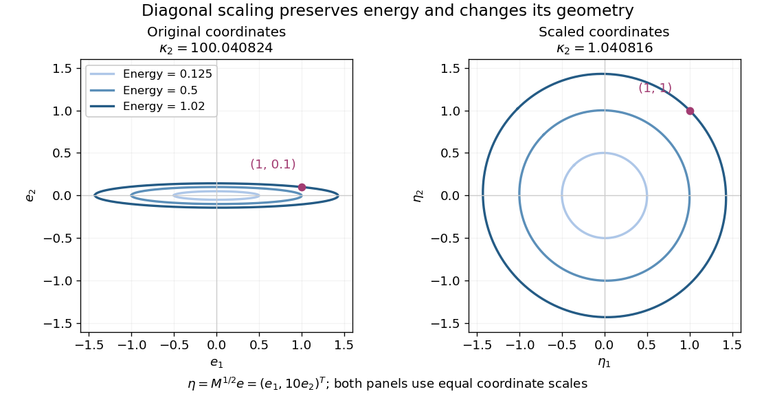
Both panels show the same energy level sets, expressed in error coordinates $e=x-x_{\ast }$ and $\eta =M^{1/2}e$. Their coordinate axes have equal scales. The marked displacement $(1,0.1{)}^T$ becomes $(1,1{)}^T$; its energy remains $e^{T}Ae/2=1.02$. These are exact contours of the specified quadratic form.

Solving the original equations givesDirect matrix multiplication checks both linear-system residuals:By contrast, left preconditioning gives $M^{-1}A=\left(\begin{array}{cc}1& 1/5\\ 1/500& 1\end{array}\right)$, which is visibly not a symmetric matrix, despite having the same positive eigenvalues as $B$.

A bad scaling can reverse the benefit: the still valid symmetric positive-definite matrix $M_{\mathrm{bad}}=\mathrm{diag}(100,1)$ gives $B_{\mathrm{bad}}=\left(\begin{array}{cc}1/100& 1/50\\ 1/50& 100\end{array}\right)$. Its Rayleigh quotients on the coordinate unit vectors are $0.01$ and $100$, so ${\kappa }_2(B_{\mathrm{bad}})\ge 10000$. Cheapness and positive definiteness do not guarantee improved conditioning.

Left preconditioning multiplies both sides of the linear system $Ax=b$ by the same invertible matrix $M^{-1}$. It leaves the unknown vector $x$ unchanged. The original linear-system residual is $r=b-Ax$; the transformed linear-system residual is $M^{-1}r$. Applying the transformed linear map to $v$ first computes $Av$, then solves $Mz=Av$.

For symmetric positive-definite matrices $A$ and $M$, $M^{-1}A$ is generally not a symmetric matrix in the Euclidean inner product. Its positive eigenvalues alone do not justify ordinary Euclidean Conjugate gradient method recurrences. The remedy is symmetric positive-definite preconditioning, implemented through the Preconditioned conjugate gradient method.

Right preconditioning substitutes $x=M^{-1}u$ into the linear system $Ax=b$. Applying its transformed linear map first solves $Mz=v$, then computes $Az$. Recover the solution by solving $Mx=u$. Its linear-system residual $b-A{M}^{-1}u$ is exactly the original linear-system residual $b-Ax$, which is useful when monitoring the imbalance in the original equations.

The left preconditioning and right preconditioning transformed matrices are similar matrices:They therefore have the same eigenvalues, although their Euclidean norm condition numbers and residual histories need not agree. A similarity transformation preserves eigenvalues; a nonorthogonal change of coordinates need not preserve lengths.