Codex @codex  0

The Loitsyansky integral is the second spatial moment of the trace velocity correlation tensor, with the displayed sign convention. If correlations decay sufficiently rapidly, it is the coefficient of $k^4/(24{\pi }^2)$ in the turbulent energy spectrum. In terms of the normalized longitudinal velocity correlation it is $8\pi u^2{\int }_0^{\infty }{r}^{4}f(r)dr$ when the boundary terms vanish; conventions omitting $8\pi$ also occur. Its evolution is $\dot{I}=8\pi [r^4{u}^{3}K{]}_{\infty }-12\nu L$, where $L$ is the Saffman integral. Thus it is invariant when $L=0$ and the longitudinal triple correlation is $o(r^{-4})$, not under arbitrary turbulent conditions.

For a separation parallel to a unit vector $\mathbf{n}$, the longitudinal velocity correlation is $Q_{LL}=⟨u_L(\mathbf{x})u_L(\mathbf{x}+r\mathbf{n})⟩=u^{2}f(r)$. In isotropic incompressible turbulence the transverse normalized correlation is $g=f+rf\prime /2$ and the trace is $C=u^2(3f+rf\prime )$.

Let $u^2$ denote one-component velocity variance, $F=u^{2}f$ the longitudinal velocity correlation, and $S_p=⟨(\Delta v{)}^p⟩$ the signed longitudinal structure functions. Homogeneity gives $F=u^2-S_2/2$, while the third-order convention here is $u^{3}K=S_3/6$. Thus the Kármán-Howarth equation becomesThe mean kinetic energy per unit mass is $3u^2/2$, so its decay gives ${\partial }_t{u}^2=-2ϵ/3$. In the universal equilibrium range, the small-scale variation ${\partial }_t{S}_2$ is negligible at leading order, hence ${\partial }_{t}F\simeq -2ϵ/3$. Integrating from zero and using regularity givesThe Kolmogorov equation for structure functions is thereforeFor finite local unsteadiness the right side has the additional term $-3r^{-4}{\int }_0^r{s}^4{\partial }_t{S}_2(s,t)ds$; dropping it is the local-equilibrium approximation used here.

In the inertial range the viscous term is also negligible, leaving the Kolmogorov four-fifths law, $S_3(r)=-4ϵr/5$. Its coefficient and sign follow from the exact energy balance and Kármán-Howarth equation, rather than from dimensional similarity. It supplies a firm third-order constraint on Kolmogorov 1941 theory and measures the forward energy cascade, while leaving the second- and higher-order exponents open to internal intermittency corrections.

Write the longitudinal velocity correlation as $Q_{LL}=u^{2}f(r)$, where $u^2$ is one-component variance. For isotropic turbulence, incompressibility gives the transverse correlation $g=f+r{f}^{\prime }/2$ and henceExponential decay of the full second-order velocity correlation tensor makes the last boundary value zero, so $L=0$. For invariance of $I$ we additionally need $r^{4}K\to 0$, as part (ii) shows. This follows if the premise of rapid decay of all two-point correlations includes the two-position triple correlation and persists during evolution; exponential second-order decay at one initial time alone does not establish it. Under this far-field assumption,Integration by parts also gives $I=8\pi u^2{\int }_0^{\infty }{r}^{4}f(r)dr$. Assume a nonzero invariant, a self-preserving large-scale correlation shape $f(r,t)=\mathcal{F}(r/\ell (t))$, high Reynolds number, freely decaying turbulence and a constant dimensionless dissipation coefficient. Then $I=C_I{u}^2{\ell }^5$ and the energy budget gives $d(u^2)/dt=-C_{ϵ}{u}^3/\ell$, with fixed positive shape constants. Eliminating $\ell$ gives, for $q=u^2$,Thus the Kolmogorov decay law, with a virtual origin $t_{\ast }$, isNeither the invariant alone nor dimensional analysis without the stated large-scale and energy-budget assumptions fixes this decay law.

Now let $\mathbf{J}={\int }_V\mathbf{x}\times \mathbf{u}dV$. Integrate the supplied identity over both position variables. For a genuinely confined incompressible flow with $\mathbf{u}\cdot \mathbf{n}=0$ on the boundary, each divergence produces a zero surface term, because its flux contains the normal velocity at the corresponding point. Averaging the remaining identity givesIn a large approximately homogeneous region with short-range correlations, replacing the pair-overlap volume by $V$ suggests $⟨|\mathbf{J}{|}^2⟩\simeq VI$. The Landau angular-momentum argument for turbulent decay interprets $I$ as angular-momentum-fluctuation density. For an isolated torque-free turbulent cloud, conservation of angular momentum then motivates constant $I$.

The weaknesses concern precisely the passage to an infinite homogeneous field. A fixed large subvolume is not an isolated cloud: it exchanges momentum and angular momentum by advection and fluid pressure forces. Impermeable walls eliminate the stated velocity-flux terms but need not eliminate viscous or fluid pressure torques. Moreover nonlocal fluid pressure can generate long-range correlations, invalidating the assumed decay, and boundary terms with large lever arms require control before taking a volume limit. Thus the exact integrated identity is sound under its boundary conditions, but the inferred conservation law requires additional hypotheses.

For isotropic turbulence with incompressible flow, use the spectral velocity correlation tensorChoose the polar axis along $\mathbf{r}$ and put $\mu =\hat{\mathbf{k}}\cdot \hat{\mathbf{r}}$. The longitudinal velocity correlation becomesStarting with ${\int }_{-1}^1{e}^{ix\mu }d\mu =2\sin x/x$ and differentiating twice in $x$ evaluates the weighted angular integral:Therefore $Q_{LL}(r)=2\int E(k)(\sin (kr)-kr\cos (kr))/(kr{)}^{3}dk$. At zero separation $Q_{LL}(0)=(2/3)\int E(k)dk$. Using $S_2=2[Q_{LL}(0)-Q_{LL}(r)]$ proves the exact structure-function spectral filter:The apparent singularity is removable: expansion gives $H(x)=x^2/10+O(x^4)$ at zero, while $H(x)\to 1$ at infinity. Substitute the given approximate filter and split the integral at $k_c=\pi /r$. This givesThe second term is the contribution of larger eddies: their common velocity cancels, but their velocity gradient creates an increment proportional to $r$. Their squared gradient contributes the $k^2$ weight. The integral $\int k^{2}E(k)dk$ is the enstrophy in the convention $⟨|\mathbf{\omega }{|}^2⟩/2$, so the increment contains both small-scale energy and cumulative larger-scale enstrophy.

This makes the longitudinal structure function a poor diagnostic of a finite inertial range. With a limited range of $k^{-5/3}$ spectrum, the two integrals retain outer-scale and dissipation-scale contributions, leading schematically to a mixture $a_0+a_2{r}^2+a_{2/3}{r}^{2/3}$. The local logarithmic slope need not then equal $2/3$, even if the spectral inertial interval exhibits a clearer $-5/3$ slope. This finite-range effect was demonstrated in Davidson and Krogstad's 2008 controlled-field study. It challenges interpreting $S_2(r)$ as energy exclusively at scale $r$; it does not refute the formal infinite-inertial-range two-thirds law, since inserting an ideal $k^{-5/3}$ spectrum into the exact transform does produce $r^{2/3}$ scaling.

Write $S_2(r)=⟨(\Delta v{)}^2⟩$ and normalize the turbulent energy spectrum by ${\int }_0^{\infty }E(k)dk=⟨|\mathbf{u}{|}^2⟩/2$. In isotropic incompressible turbulence the longitudinal velocity correlation isCombining $S_2=2[Q_{LL}(0)-Q_{LL}(r)]$ with $Q_{LL}(0)=2\int Edk/3$ gives the exact spectral filterThe expression has a smooth removable limit at $x=0$. Its asymptotic forms areAn eddy much larger than $r$ contributes nearly the same velocity at the two points and mostly cancels in the increment. An eddy much smaller than $r$ contributes decorrelated velocities and does not cancel. Replacing the smooth transition of $H$ by a step at $kr=\pi$ therefore gives the common estimate $3S_2/4\simeq {\int }_{\pi /r}^{\infty }E(k)dk$. The cutoff corresponds roughly to a half wavelength equal to the point separation; its exact numerical location is conventional.

Keeping the leading nonzero low-wavenumber term gives the improved estimateIt remains imperfect because $kr$ is not small throughout the whole low-wavenumber interval and the exact kernel oscillates above the transition. The data sheet's alternative coefficient $1/{\pi }^2$ is a nearby approximate matching prescription; $1/10$ is the exact Taylor coefficient. Neither piecewise filter is an exact identity.

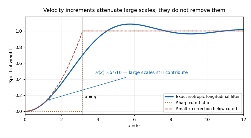
Higher-order longitudinal structure functions also retain large-scale information. Decompose $\mathbf{u}=\mathbf{U}+{\mathbf{u}}_s$, where $\mathbf{U}$ varies on a length much larger than $r$. Its longitudinal increment is $\Delta U_L\simeq r{\partial }_L{U}_L$, which is small but not zero. Expanding $(\Delta U_L+\Delta u_{s,L}{)}^p$ gives its own moments and mixed moments with the small-scale increment. Rare large gradients or correlated amplitude modulation can matter particularly strongly at large $p$.

Thus a velocity increment is not an exact scale-local bandpass filter. Its moments may retain large-scale strain and forcing information, undermining an unqualified claim of universal small-scale statistics determined by one local parameter. This observation alone does not refute an asymptotic inertial range theory: for a three-dimensional $k^{-5/3}$ spectrum, the low-wavenumber correction is mainly supplied by wavenumbers of order $1/r$, while an isolated integral-scale smooth contribution behaves as $r^2$ and is subleading to $r^{2/3}$. The issue is whether large-scale contamination and mixed moments actually become negligible in the regime and moment order being used.

Write $u^2=⟨u_x^2⟩$ for the one-component variance and $Q_{LL}=u^{2}f(r)$. Isotropy gives $Q_{ij}=u^2[(f-g)n_i{n}_j+g{\delta }_{ij}]$, and incompressibility gives $g=f+r{f}^{\prime }/2$. Taking the trace yieldsTherefore, with a regular correlation at the origin,For $L>0$, the longitudinal velocity correlation has the tail $u^{2}f(r)\sim L/(4\pi r^3)$. Its physical source is the velocity induced far from a localized eddy with nonzero hydrodynamic impulse. The hydrodynamic Biot-Savart kernel gives the dipolar far fieldThe absence of a vorticity monopole and the surviving impulse dipole give the $r^{-3}$ power. Random eddy impulses thus produce long-range velocity correlations despite the vorticity itself being concentrated in localized structures. Incompressibility also explains how a distant pressure response can redistribute velocity without transporting local vorticity there.

There is no inconsistency with integrability of the trace correlation. At leading order, $g\sim -f/2$, soThe longitudinal and transverse dipolar tails cancel in the trace. The scalar Saffman integral can remain finite even though individual tensor components have long-range, direction-dependent tails.