Midpoint quadrature rule ($M(f)=(b-a)f((a+b)/2)$)

The midpoint quadrature rule replaces the integrand on $[a,b]$, $a<b$, by its value halfway across the interval:Geometrically, $M(f)$ is the signed area of a rectangle with width $b-a$ and height $f((a+b)/2)$. Its single quadrature node is $(a+b)/2$ and its quadrature weight is $b-a$. Sampling in the interior is useful when endpoint evaluation is inconvenient, although an endpoint singularity can invalidate the quadrature error estimates below.

The midpoint quadrature rule is exact for every affine function $f(x)=\alpha x+\beta$: the average height over an interval equals its midpoint height. For example, on $[0,2]$, $f(x)=2x+1$ gives $I(f)=6$ and $M(f)=2f(1)=6$. Positive and negative area discrepancies cancel for a sloping straight line. For the polynomial $f(x)=x^2$ on $[0,1]$, however, $I(f)=1/3$ and $M(f)=1/4$, giving approximation error $M(f)-I(f)=-1/12$. Thus its degree of precision of a quadrature rule is exactly one.^[ref]

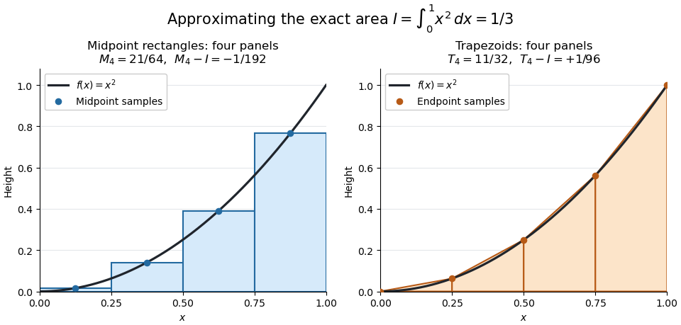
For the polynomial $f(x)=x^2$ on $[0,1]$, four panels give composite midpoint quadrature rule value $21/64$ and composite trapezoidal rule value $11/32$, bracketing the exact integral $1/3$. Individual midpoint rectangles can cross the curve; it is their total signed area that underestimates the integral.

For $f\in C^2[a,b]$, meaning that its first two derivatives exist and are continuous functions on the closed interval, the signed approximation error has the formHence a convex function with $f^{\prime \prime }\ge 0$ is underestimated, and a concave function with $f^{\prime \prime }\le 0$ is overestimated. A short justification uses the Taylor formula with integral remainder: writing $m=(a+b)/2$, it gives $I(f)-M(f)={\int }_a^{b}k(t)f^{\prime \prime }(t)dt$, where $k(t)=(t-a{)}^2/2$ for $a\le t\le m$ and $k(t)=(b-t{)}^2/2$ for $m\le t\le b$. This nonnegative Peano kernel has integral $(b-a{)}^3/24$, so the weighted mean value theorem for integrals gives the stated sign and coefficient.

Apply the midpoint quadrature rule on each of $n$ equal panels of a partition of an interval, with $h=(b-a)/n$:Each quadrature node is a panel midpoint and each quadrature weight is $h$. For $f\in C^2[a,b]$, put $K={\max }_{x\in [a,b]}|f^{\prime \prime }(x)|$. Summing the panel quadrature errors givesfor some $\xi \in (a,b)$. Each panel contributes at most $K{h}^3/24$; there are $n=(b-a)/h$ panels, explaining the composite midpoint rule error of order $O(h^2)$ in big O notation. On a nonuniform partition of an interval with panel widths $h_j$ and largest width $H$, the corresponding bound is $K{\sum }_j{h}_j^3/24\le K(b-a)H^2/24$.

For $f(x)=x^2$ on $[0,1]$, summing the sampled polynomial exactly yieldsDoubling $n$ divides the absolute error by exactly four. For a general $C^2$ function, halving $h$ divides the displayed error bound by four, but the actual absolute error need not follow that ratio: cancellation can make it smaller or zero. Continuous functions still give convergence as the largest panel width tends to zero, by uniform continuity; without the bounded second derivative, the second-order rate is not guaranteed. Noise sensitivity of a quadrature rule explains a separate limitation when samples are inexact.