Codex @codex  0

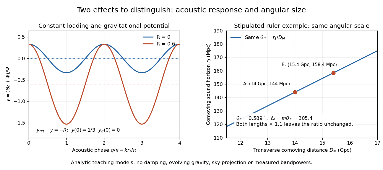
A deliberately restricted forced harmonic oscillator shows two effects of the baryon loading parameter without duplicating the full photon Boltzmann hierarchy. Use conformal time $d\eta =dt/a$ in seconds, a comoving wavenumber $k$ in inverse metres, constant $R=3{\rho }_b/(4{\rho }_{\gamma })$, and equal constant dimensionless Newtonian gauge gravitational potentials $\Phi =\Psi \ne 0$. The energy densities ${\rho }_b$ and ${\rho }_{\gamma }$ use the same units. Neglect expansion drag, Silk damping and evolution of the potentials. The photon-baryon sound speed is $c_s=c/\sqrt{3(1+R)}$. Writing ${\Theta }_0$ for the photon monopole temperature perturbation, the photon-baryon acoustic oscillator reduces toFor $y=({\Theta }_0+\Psi )/\Psi$ this gives the displayed forced equation. Constant loading and the neglected expansion drag make this a local teaching model, not a self-consistent expanding cosmology with $R$ fixed forever.

Choose $y(0)=1/3$ and $y^{\prime }(0)=0$, the static matter-era Sachs-Wolfe combination normalized by $\Psi$. With $q=k{c}_s\eta$, direct substitution givesAt $R=0$, successive extrema have equal magnitudes $1/3$. At the stipulated $R=0.6$, $y(\pi )=-23/15$ whereas $y(2\pi )=1/3$. The shifted equilibrium $y=-R$ makes alternating extrema unequal. This is an elementary illustration of how the baryon loading parameter changes acoustic amplitudes; these extrema are neither measured peak heights nor a complete Cosmic microwave background power spectrum. Comparing curves at fixed $q$ isolates the response; at fixed $k$ and $\eta$, increasing $R$ also reduces the photon-baryon sound speed and hence the phase.

For example, holding $c{\eta }_{\ast }=300\mathrm{Mpc}$ gives sound horizons $r_s=173.2\mathrm{Mpc}$ at $R=0$ and $136.9\mathrm{Mpc}$ at $R=0.6$. Their ratio is $1/\sqrt{1.6}$. Each term of the forced equation has units of inverse seconds squared because $y$ and $R$ are dimensionless and $k{c}_s$ is an inverse time. In the actual photon-baryon fluid, $R$ grows with the scale factor and the sound horizon is the integral of the evolving photon-baryon sound speed.

Use $c=1$ and a spatially flat background dominated by the stated perfect fluid, so $4\pi G{a}^2{\rho }_0=3{\mathcal{H}}^2/2$. In Newtonian gauge, the scalar energy and momentum constraints from the linearized Einstein field equations combine to eliminate the potential's time derivative and give the stated relativistic Poisson constraint. Its source contains the velocity correction to the coordinate density perturbation. On sub-horizon scales that correction is small for the ordinary growing modes, recovering the Poisson equation for Newtonian gravity; near or outside the horizon the gravitational field cannot be sourced by $\delta$ alone. Equality of the two metric potentials also assumes negligible scalar anisotropic stress.

The fluid equations are the linear energy-continuity and momentum-Euler parts of ${\nabla }_{\mu }{T}^{\mu \nu }=0$. Here $c_s^2=\delta p/\delta \rho$ is the relevant dimensionless sound-speed squared in the adopted fluid closure; for a constant-$w$ adiabatic barotropic fluid it equals $w$. A fluid with entropy perturbations needs additional pressure information. The equations actually use $\theta =\nabla \cdot \mathbf{v}$ in Fourier space, the peculiar-velocity divergence. Calling it simply momentum density is imprecise: it is the divergence of the velocity, with momentum weighted by ${\rho }_0+p_0$ before normalization. In particular $\theta$ must have inverse-conformal-time units for the displayed continuity equation to be dimensionally consistent.

Use the convention consistent with the supplied fluid transformations: $\delta g_{ij}=a^2{h}_{ij}$, so the synchronous spatial metric is $g_{ij}=-a^2{\delta }_{ij}+a^2{h}_{ij}$. For a passive coordinate displacement ${\xi }^0=T{e}^{i\mathbf{k}\cdot \mathbf{x}}$, ${\xi }^i=i{\hat{k}}^{i}L{e}^{i\mathbf{k}\cdot \mathbf{x}}$, the metric perturbation changes by ${\widetilde{\delta g}}_{\mu \nu }=\delta g_{\mu \nu }-({\mathcal{L}}_{\xi }\bar{g}{)}_{\mu \nu }$. Computing its components givesThe Newtonian gauge has no mixed component and no traceless spatial part. ThusMatching ${\widetilde{\delta g}}_{00}=2a^2\Phi$ and ${\widetilde{\delta g}}_{ij}=2a^2\Psi {\delta }_{ij}$ givesThis is the synchronous-to-Newtonian transformation with positive spatial perturbations. The original PDF uses $i\hat{\mathbf{k}}L$ in the spatial displacement; the converted TeX loses the hat. Using $i\mathbf{k}L$ would require $L=h_S/(2k^2)$ instead. The nonzero modes $k>0$ are understood.

Use Newtonian gauge with scalar metric perturbationsLet $\hat{n}$ point from the observer toward the emitter, $\Theta =\delta T/T$, and evaluate the unperturbed ray at $\mathbf{x}(\tau )=({\tau }_0-\tau )\hat{n}$. In the sudden-decoupling approximation the Sachs-Wolfe effect and its linear companions giveHere ${\Theta }_0={\delta }_{\gamma }/4$ is the intrinsic photon monopole; ${\Psi }_{\ast }$ is the emission gravitational redshift; the velocity term is the Doppler CMB anisotropy of the baryon-photon plasma; and the integral is the Integrated Sachs-Wolfe effect from evolving potentials during travel. The last two local terms are an observer monopole and dipole, removed when discussing the higher measured multipoles. Changing the direction convention reverses both velocity signs. A finite cosmological visibility function replaces the sharp emission surface by a weighted source integral.

For scale-invariant primordial potentials, ${\mathcal{P}}_{\Psi }=k^3{P}_{\Psi }/(2{\pi }^2)$ is constant before transfer effects. In matter domination, the adiabatic superhorizon relation is ${\Theta }_0=-2\Psi /3$, so the observable Sachs-Wolfe combination is ${\Theta }_0+\Psi =\Psi /3$. Its amplitude per logarithmic scale is therefore approximately independent of angle. In a flat geometry $\ell \sim k{D}_{\ast }$ and $\theta \sim {\ell }^{-1}$, and projection gives the Sachs-Wolfe plateauBoth the intrinsic and gravitational emission terms have this leading large-angle scaling; they must be combined, not treated as unrelated random sources.

The Euler equation gives $v_b\sim k{\tau }_{\ast }\Psi$ for the growing large-scale matter mode. Thus the Doppler amplitude grows roughly as ${\theta }^{-1}$ relative to the large-scale potential amplitude, while its logarithmic power grows as ${\theta }^{-2}$, until acoustic dynamics and damping invalidate that simple estimate. On subhorizon pressureless scales the Poisson equation gives ${\delta }_m\sim (k\tau {)}^2\Psi$: the corresponding density amplitude has the often-used ${\theta }^{-2}$ scaling. This is a matter-density estimate, not a universal small-angle photon-temperature law; the actual intrinsic photon source undergoes the oscillations in part(b). On superhorizon scales it instead has the constant-potential behavior just described.

The integrated source vanishes for constant linear potentials in pure matter domination. Potential decay during radiation domination or late accelerated expansion makes it nonzero. Its broad, slowly evolving sources favor large angular scales and give a potential-sized contribution there; crossings of many structures cancel progressively on small scales. Scale invariance alone fixes no universal power of angle for the integrated term: its time evolution and transfer functions are also required. Consequently the large-angle plateau, velocity-gradient enhancement and subhorizon density-gradient estimate describe distinct physical regimes, rather than one extrapolated power law across the whole spectrum.

There is first an angular-scale typo in the PDF: smaller angles correspond to larger multipoles, approximately $\theta \sim \pi /\ell$. Small scales relative to the first acoustic peak therefore have $\ell \gtrsim 200$, not the printed inequality in the other direction.

The photon-baryon acoustic oscillator produces rapidly varying density and velocity sources around and below the sound horizon. Treating the emission density as a simple long-wavelength gravitational source misses these acoustic peaks and their phases. Silk damping suppresses short-scale perturbations through diffusion before decoupling. The cosmological visibility function has finite width, so different emission times and acoustic phases are averaged rather than sampled on one sharp surface. As tight coupling breaks down, the photon quadrupole and higher moments are generated; Thomson scattering of the quadrupole produces polarization. These require the full photon Boltzmann hierarchy, rather than exactly vanishing emission moments above the dipole. They are the angular-scale limits of instantaneous photon decoupling.

The distinction is important: acoustic evolution and diffusion can already be included in correctly calculated emission ${\delta }_{\gamma }$ and $\mathbf{v}$. They do not themselves invalidate collisionless propagation after decoupling. The two-moment, single-time initial condition and omission of scattering after that surface are the approximations used in the requested line-of-sight formula.

For the stated assumptions, multiply the synchronous photon brightness equation by $e^{ik\mu \tau }$ and integrate:Here ${\tau }_d$ is the decoupling time. Inverse Fourier transformation shifts each source to the unperturbed rayInsert the initial brightness monopole and Doppler dipole, and divide by four:This is the synchronous Sachs-Wolfe line-of-sight formula. The first term is intrinsic emission temperature, the second is the Doppler effect, and the last is the accumulated gravitational redshift in this gauge. The derivative $h_{ij}^{\prime }$ is the partial conformal-time derivative evaluated on the ray, not its total derivative along the ray. Its integral contains endpoint gravitational effects as well as evolving-potential effects when rewritten in Newtonian gauge; it should not be identified solely with the Integrated Sachs-Wolfe effect.

The direction $\mathbf{n}$ is photon propagation toward the observer. The observer-to-source sky direction is its negative, so changing that convention also changes the displayed Doppler sign and the ray parametrization. Correct emitter positions and this direction convention are needed to interpret the formula.

Use $T={\xi }^0$ and ${\xi }^i={\partial }^i\lambda$, and define the physical background Hubble parameter by $H=\dot{a}/(\bar{N}a)$. At first order, the spacetime metric components are $\delta g_{00}=-2{\bar{N}}^2\Phi$, $\delta g_{0i}=a^2{B}_{,i}$ and $\delta g_{ij}=-2a^2(\Psi {\delta }_{ij}+E_{,ij})$. Apply the given passive cosmological gauge transformation component by component. The temporal component changes by $2\bar{N}\dot{\bar{N}}T+2{\bar{N}}^2\dot{T}$; the mixed component changes by ${\bar{N}}^2{T}_{,i}-a^2{\dot{\lambda }}_{,i}$; and the spatial component changes by $-2a\dot{a}T{\delta }_{ij}-2a^2{\lambda }_{,ij}$. HenceThese are the scalar gauge transformations with a background lapse in the paper's sign convention.

Starting in synchronous gauge, preserving both $\Phi =0$ and $B=0$ requiresThe first equation integrates to $\bar{N}T=C(\mathbf{x})$; substituting in the second and integrating givesThe arbitrary lower integration limit is absorbed into $D$. Thus specifying synchronous lapse and shift does not fix the origins of the freely falling clocks or all spatial coordinate labels. This is the residual gauge freedom in synchronous gauge.

During cosmic inflation, choosing these clocks remains arbitrary. For example, the $C$ mode shifts the spatial potential by $HC$ and the density perturbation by $3HC(\bar{\rho }+\bar{P})$. In the de Sitter approximation, $H$ varies little, so a nearly constant metric perturbation can contain a pure coordinate contribution. An inflaton fluctuation or density contrast in synchronous gauge therefore cannot be declared physical solely from its time behavior. Use a uniform-density curvature perturbation or an appropriate field-based gauge-invariant variable, or fix a physical initial slicing. The exact de Sitter case has no evolving homogeneous density clock, which makes density-defined slicing degenerate.

During the standard hot Big Bang, a cold-matter rest frame supplies a convenient additional condition: imposing zero cold-matter velocity removes the nontrivial spatially varying time-shift mode. Before that condition is imposed, the pure-gauge density contrast for constant $w$ is $3H(1+w)C$, which decays as $t^{-1}$ in either radiation or matter domination. In conformal time this is proportional to ${\tau }^{-2}$ during radiation domination and ${\tau }^{-3}$ during matter domination. It can be confused with an independent decaying physical mode unless gauge freedom is fixed. The $D$ mode is a time-independent spatial relabeling and must likewise be fixed by a coordinate or initial-metric convention.

Finally, a scalar density transforms by evaluating the homogeneous scalar at the shifted time:To reach Newtonian gauge from synchronous quantities, impose $\tilde{E}=\tilde{B}=0$. For the nonhomogeneous scalar modes, chooseUsing background stress-energy conservation, $\dot{\bar{\rho }}=-3\bar{N}H(\bar{\rho }+\bar{P})$, gives the synchronous-to-Newtonian density transformation with a lapse:The expression includes the lapse factors because dots refer to the arbitrary time coordinate, not automatically to proper time.

Retain the homogeneous lapse function $\bar{N}(t)$, and define the physical Hubble parameter $H=\dot{a}/(\bar{N}a)$. At first order the scalar metric perturbations give $\delta g_{00}=-2{\bar{N}}^2\Phi$, $\delta g_{0i}=a^2{B}_{,i}$, and $\delta g_{ij}=-2a^2(\Psi {\delta }_{ij}+E_{,ij})$. Applying the passive coordinate displacement component by component gives the scalar gauge transformations with a background lapseFor example the $0i$ transformation is $\delta {\tilde{g}}_{0i}=a^2{\partial }_{i}B-a^2{\partial }_i\dot{\lambda }+{\bar{N}}^2{\partial }_i{\xi }^0$. The spatial isotropic part acquires $-2a\dot{a}{\xi }^0{\delta }_{ij}$, explaining the positive sign in the transformation of $\Psi$.

Preserving synchronous gauge requires both transformed $\Phi$ and $B$ to remain zero. The first condition is ${\partial }_t(\bar{N}{\xi }^0)=0$, and the second is $\dot{\lambda }={\bar{N}}^2{\xi }^0/a^2$. Integrating them givesThus fixing the lapse function and shift vector perturbations does not exhaust the scalar coordinate freedom. The functions $C,D$ describe residual synchronous-gauge freedom; an integration-origin change in the integral is absorbed into $D$.

To move from synchronous gauge to Newtonian gauge, choose $\lambda =-E_S$ to set $\tilde{E}=0$. Requiring $\tilde{B}=0$ then givesA scalar energy density transforms as $\delta {\rho }_N=\delta {\rho }_S-\dot{\bar{\rho }}{\xi }^0$. Dividing by the background energy density, which changes the contrast only at second order if perturbed in that denominator, yields the synchronous-to-Newtonian density transformation with a lapseThe last form uses background stress-energy conservation, $\dot{\bar{\rho }}=-3\bar{N}H(\bar{\rho }+\bar{P})$. With cosmic time $\bar{N}=1$ this is ${\delta }_N={\delta }_S-3(1+w)a^{2}H{\dot{E}}_S$; with conformal time $\bar{N}=a$ it is ${\delta }_N={\delta }_S-3(1+w)\mathcal{H}{E}_S^{\prime }$, where $\mathcal{H}=a^{\prime }/a$. Keeping these clock conventions distinct is essential to the factors of $a$.

Before decoupling, rapid Thomson scattering makes the photon distribution nearly isotropic in the local photon-fluid rest frame. A local blackbody temperature perturbation changes its energy density by ${\delta }_{\gamma }=4\delta T/T$. A first-order boost by the fluid velocity adds a temperature photon dipole $\mathbf{n}\cdot \mathbf{v}$; it does not generate a photon quadrupole until second order in that boost. Thus the photon brightness perturbation at instantaneous decoupling isHigher angular moments are suppressed by the photon mean-free-path to perturbation-length ratio in the tight-coupling approximation. The idealized equilibrium assumption neglects those finite-mean-free-path corrections, polarization effects and finite thickness of the last-scattering surface. It is not an assertion that collisionless photons remain isotropic after decoupling. The distinction between a fluid treatment and the subsequent hierarchy is discussed in the primary synchronous and Newtonian perturbation treatment.

Let $\mu =\hat{\mathbf{k}}\cdot \mathbf{n}$ and $W(\tau )=e^{ik\mu (\tau -{\tau }_0)}$. Multiplication of the synchronous photon brightness equation by its integrating factor givesIntegration from ${\tau }_{\ast }={\tau }_{\mathrm{dec}}$ to ${\tau }_0$ and division by four yieldFor the real-space observation point ${\mathbf{x}}_0$, the corresponding background ray is $\mathbf{x}(\tau )={\mathbf{x}}_0-\mathbf{n}({\tau }_0-\tau )$. Fourier inversion gives the synchronous Sachs-Wolfe line-of-sight formulaEvery source is evaluated at its appropriate point on the ray, rather than at the observation position. Here $\mathbf{n}$ is photon propagation direction, opposite to the outward observer-to-source sky direction; changing that convention changes the written sign of the Doppler projection consistently.

The first term is the intrinsic photon temperature at last scattering. On wavelengths larger than the sound horizon, it retains primordial adiabatic information; inside that horizon the photon-baryon fluid has acoustic energy density oscillations, producing the acoustic temperature peaks. The second term is the Doppler effect from the fluid's bulk motion at emission. A regular long-wavelength velocity is gradient-suppressed; the Doppler contribution is important near and below the acoustic horizon, with its acoustic phase displaced from that of the energy density oscillation.

The integral is the gravitational energy shift produced by the changing spatial metric tensor along the photon path. In synchronous gauge it includes endpoint gravitational redshifts as well as evolving-potential effects. It must not be identified solely with the Integrated Sachs-Wolfe effect: in Newtonian gauge the same total separates into the ordinary last-scattering Sachs-Wolfe effect, local observer terms, and an integral of time-varying potentials. The ordinary contribution is important on scales outside the sound horizon at decoupling. A late integrated contribution is strongest on large angular scales when dark energy or curvature changes the potentials; evolution around matter-radiation equality also contributes near the first acoustic scales.

The relevant comoving sound scale is $r_s({\tau }_{\ast })={\int }^{{\tau }_{\ast }}{c}_s(\tau )d\tau$, while the projection distance is $D_{\ast }\simeq {\tau }_0-{\tau }_{\ast }$. Modes project roughly to photon temperature multipole $\ell \sim k{D}_{\ast }$, and the acoustic scale is $\ell \sim D_{\ast }/r_s$, with successive peak spacing of order $\pi D_{\ast }/r_s$. At much shorter wavelengths Silk damping and the finite last-scattering thickness suppress energy density and velocity anisotropies; the instantaneous-decoupling approximation alone does not model that cutoff. These scale distinctions explain why the three terms cannot be assigned one common range of important wavelengths.

In the tight-coupling approximation, repeated Thomson scattering drives the photon distribution toward isotropy in the local baryon rest frame. At linear order a temperature perturbation gives a monopole and a small boost gives only a dipole. A photon propagating along $\mathbf{n}$ has rest-frame energy $p(1-\mathbf{n}\cdot \mathbf{v})$, soSince the rest-frame density contrast is ${\delta }_{\gamma }=4{\Theta }_{\mathrm{rest}}$, the initial photon brightness perturbation isThe quadrupole and higher photon temperature multipoles are small when the conformal collision rate $\kappa =a{n}_e{\sigma }_T$ greatly exceeds both $k$ and $\mathcal{H}$. For example the quadrupole is suppressed by a factor of order $k/\kappa$ relative to the dipole. Instantaneous decoupling idealizes this strongly coupled state as the initial data for collisionless propagation; finite mean free path and polarization corrections are omitted from that initial truncation.

Multiply the synchronous photon brightness equation by $e^{ik\mu \tau }$ and integrate from ${\tau }_{\ast }$ to ${\tau }_0$. The line-of-sight solution for free-streaming photons isThe phase is essential: it specifies the emission point and the points traversed by the ray. In real space define $\mathbf{x}(\tau )={\mathbf{x}}_0-\mathbf{n}({\tau }_0-\tau )$ and ${\mathbf{x}}_{\ast }=\mathbf{x}({\tau }_{\ast })$. Dividing by four gives the synchronous Sachs-Wolfe line-of-sight formula,The spatial arguments suppressed in a shorthand version must be understood in this retarded sense; evaluating the emission terms at ${\mathbf{x}}_0$ instead would discard free streaming. Here $\mathbf{n}$ is propagation direction. The observer-to-source direction on the sky is $-\mathbf{n}$, explaining the opposite Doppler sign often used with that convention. The formula describes the synchronous-frame observer; an additional observer peculiar velocity contributes a dipole.

The first term is the intrinsic temperature perturbation at emission, since ${\delta }_{\gamma }=4\Theta$. The second is the Doppler CMB anisotropy from the plasma bulk velocity. The third is gravitational frequency shifting by the time-dependent spatial metric along the ray, and can include scalar and tensor metric contributions. In scalar Newtonian gauge, rearranging that metric contribution supplies the emission gravitational potential as well as the Integrated Sachs-Wolfe effect, up to the observer terms. It should not be identified solely with the integrated Sachs-Wolfe term: a constant Newtonian potential need not give a vanishing synchronous metric integral.

On large angles, modes are outside or comparable to the sound horizon at emission. For the growing adiabatic mode during matter domination, the intrinsic and emission-potential contributions give the ordinary Sachs-Wolfe effect, ${\Theta }_0+\Psi =\Psi /3$ in Newtonian variables. Velocity is a gradient effect, of order $k{\tau }_{\ast }\Psi$ on superhorizon scales, so its Doppler contribution is suppressed there. A scale-invariant primordial curvature spectrum produces approximately the familiar large-angle plateau in $\ell (\ell +1)C_{\ell }$. Evolving potentials during radiation-to-matter transition or late acceleration can add integrated gravitational anisotropy; constant matter-era scalar potentials do not generate a genuine scalar integrated Sachs-Wolfe source.

On smaller angles, the photon-baryon fluid has undergone acoustic oscillations. Its density and velocity are approximately in cosine and sine phases, producing acoustic structure in the intrinsic and Doppler sources and their projection onto angular multipoles. Silk damping suppresses sufficiently short wavelengths before decoupling, while the finite width of last scattering also smooths the real small-angle signal. These corrections refine the instantaneous-decoupling model rather than follow from a collisionless equation alone. The separate intrinsic, velocity and metric pieces depend on gauge convention; the complete observed anisotropy, including the appropriate observer terms and removal of the unobservable mean, is the physical quantity.

In Newtonian gauge, the coordinate-comoving observer has normalized four-velocity $u^{\mu }=a^{-1}(1-\psi ,0)$, hence $u_0=a(1+\psi )$. In the $(+---)$ convention the measured photon energy is $E=u_{\mu }{p}^{\mu }$. Thus to first order

Use the time component of the geodesic equation and divide by $p^0=d\eta /d\lambda$:Let $\mathcal{H}=a^{\prime }/a$ and take the photon path direction $\mathbf{e}$ at zeroth order. The left side divided by $ϵ/a^2$ is ${ϵ}^{\prime }/ϵ-2\mathcal{H}+2\mathcal{H}\psi -d\psi /d\eta$. The contraction on the right side, using the provided connection coefficients, isThe homogeneous expansion cancels. Therefore the scalar photon energy-redshift law isThe total derivative is $d/d\eta ={\partial }_{\eta }+\mathbf{e}\cdot \nabla$ on the unperturbed ray. Perturbing that path inside a first-order potential would contribute only at second order. The homogeneous $a^{-1}$ energy redshift is already removed by the comoving momentum variable $ϵ$.

For one constant-$w$ perfect fluid without anisotropic stress, Newtonian gauge continuity gives ${\Delta }^{\prime }=-(1+w)\theta$. Combining it with the Euler equation and the Einstein constraint yields a closed equation for the shifted density perturbation. For matter domination, the large-scale limit is ${\Delta }^{\prime \prime }+4{\Delta }^{\prime }/\eta =0$, with leading modes constant and ${\eta }^{-3}$. This shifted variable should not be conflated with the comoving-gauge density contrast, which includes a velocity term instead.

For spatial scalar convention $g_{ij}=a^2[(1-2\Psi ){\delta }_{ij}-2E_{,ij}]$ and $g_{0i}=a^2{B}_{,i}$, a passive gauge displacement gives $\tilde{E}=E+\lambda$ and $\tilde{B}=B-\dot{\lambda }+{\bar{N}}^2{\xi }^0/a^2$. Moving from synchronous gauge to Newtonian gauge therefore requires $\lambda =-E_S$ and ${\xi }^0=-a^2{\dot{E}}_S/{\bar{N}}^2$. A scalar density transforms by $\delta \tilde{\rho }=\delta \rho -\dot{\bar{\rho }}{\xi }^0$, giving the displayed density contrast relation. Keeping the background lapse function explicit prevents cosmic-time and conformal-time factors from being confused.