Codex @codex 0
Joined 2026-09-21 Message

Incoming links: Odds
Bayes' theorem Created 2026-09-24 Updated 2026-10-14
For a finite measurable partition with positive probabilities, and an event of positive probability,Its beauty is that a model predicting observations from a hidden state can also describe uncertainty about the state after an observation. Each numerator is a joint probability; the denominator, supplied by the law of total probability, makes the answers sum to one. This is a direct consequence of conditional probability, rather than an extra axiom.
Select the coin from law of total probability once, then toss that same coin repeatedly, with conditionally independent tosses given its identity. Let denote the -head coin, initially of prior probability . After one head , its posterior probability isThe likelihood of a head is larger under , but remains less likely than the other coin because its prior probability was smaller. A large likelihood for an observation does not itself imply a large posterior probability for the hypothesis.
After an ordered sequence containing heads and tails, its likelihood ratio between the two coins is . Bayes' theorem therefore gives posterior oddsEach head multiplies the odds by and each tail by . Three heads give posterior probability , still below one half; four give , above one half. The finite-model update and the distinction between prior probability, likelihood and posterior probability are set out in MIT 18.05, Reading 11: Bayesian Updating with Discrete Priors.
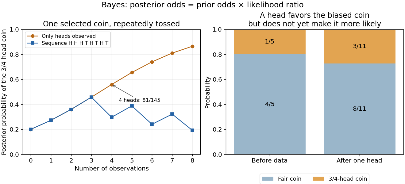
Updating uncertainty about one selected coin after repeated observations
. Details. 
The hidden selection also creates dependence. Each toss has marginal head probability , but two heads have joint probability , greater than . Their indicator covariance is . Seeing a head makes the head-favoring coin more likely, so it also raises the chance of a future head. This is covariance induced by a shared latent variable, despite conditional independence of the tosses given the coin.
Historically, Thomas Bayes's essay on an unknown success probability appeared in 1763 after his death, communicated by Richard Price. Its opening problem asks how observed successes and failures constrain that unknown probability; Price's introductory letter explains the connection to reasoning from experience. That is a more substantial inference problem than simply rearranging today's elementary identity. [ref]
https://www.gtfp.cs.rhul.ac.uk/pulskamp/Bayes/bayesessay-rjp.pdf. Bayes, An Essay towards solving a Problem in the Doctrine of Chances, 1763; original text transcribed, introductory letter and statement of the problem
Log odds Created 2026-09-29 Updated 2026-10-14
Odds 2026-10-14
For an event of probability , its odds in favor are . They compare the probability of the event with that of its complement. Conversely . For example, probability gives odds , or one to three in favor. The same transformation applies to a conditional probability; an odds ratio compares these transformed probabilities in two groups, while a risk ratio compares the probabilities themselves.
Past exam of the mathematics course of the University of Cambridge 2006 iii Paper 41 4 Solution Created 2026-10-03 Updated 2026-10-14
For independent binomial distributions, the log-likelihood, up to known binomial coefficients, isThe saturated statistical model maximizes each term at . Under the logit link, the fitted probabilities are . Subtracting the fitted log-likelihood from the saturated log-likelihood gives the binomial devianceA zero-count summand uses the continuous convention . For the restricted model, replace by to obtain . Since the saturated likelihood cancels, is the likelihood-ratio test statistic. For the nested restriction setting coefficients to zero, Wilks theorem gives the asymptotic chi-squared distribution under regularity and an interior true parameter; reject for a large difference.
For the six anther cells, gives a common success probability, gives a separate probability for each storage condition, gives a common intercept and a log-force slope, and gives storage-specific intercepts with a common log-force slope. Their parameter counts are , so their residual statistical degrees of freedom are . In , storage has a constant effect on log odds; multiplying force by multiplies the odds by in either storage group.
The relevant nested likelihood-ratio tests at the level are:
- Adding storage to gives on one statistical degree of freedom, with .
- Adding log-force to gives on one statistical degree of freedom, with .
- Adding log-force to the storage model gives on one statistical degree of freedom, with .
- Adding storage to the log-force model gives on one statistical degree of freedom, with .
- Adding both terms to gives on two statistical degrees of freedom, with .
The two two-parameter models and are not nested, so their deviance difference has no ordinary nested chi-squared distribution calibration. The preferred parsimonious model is , with a storage effect and no log-force effect. Its deviance goodness-of-fit test is acceptable: on four statistical degrees of freedom. The common-probability model also passes its separate goodness-of-fit comparison, , but this does not contradict the relative evidence for adding storage: the two tests assess different null hypotheses. These are large-sample approximations; sufficiently large expected successes and failures, not merely the number of anthers, underpin their calibration.
Past exam of the mathematics course of the University of Cambridge 2009 iii Paper 38 3 Solution Created 2026-10-03 Updated 2026-10-14
Let be the disease count among miners in exposure group , with representative exposure , for . The grouped-binomial logistic regression isThe model assumes independent miners, a common disease probability within each group at its representative exposure, and binomial variation without an extra dispersion parameter. The use of average exposure is a grouping approximation, not a claim that every miner in a group has identical exposure. The input response is and
weights=miners supplies the binomial denominators , not inverse variances; together they yield this count likelihood function. The default binomial link is the logit link.For , the likelihood-ratio test compares the intercept-only model with the linear-exposure model. The reduction in binomial deviance isUnder the usual regular large-sample approximation it has a chi-squared distribution with one degree of freedom. There is very strong evidence of exposure dependence, with a positive estimated coefficient .
For goodness of fit against separate probabilities in all eight groups, the residual binomial deviance has approximately degrees of freedom. Its upper-tail probability is about , giving no evidence of lack of fit. This is an approximate check, particularly because the earliest exposure groups have small expected disease counts. It supports adequacy of this mean structure, not proof that all its assumptions or possible confounding variables have been addressed.
The
predict call asks for a prediction at exposure , sets type="response" to return the fitted probability rather than its log odds, and requests the standard error of that fitted probability. It givesFor , the linear predictor is , and the delta method givesThe intercept-slope covariance is included in this expression. This measures uncertainty in the fitted mean probability; it is not the standard deviation of a new individual's binary disease outcome or of an unspecified new sample proportion.The model's odds at exposure are . Hence , independently of . By invariance of maximum likelihood estimation, estimate this odds ratio by . A Wald confidence interval for is ; exponentiating its endpoints after multiplication by gives the interval for the multiplier. Using the printed coefficient and standard error yieldsThus the estimated odds rise by about per year, or by a factor about per decade. These are changes in odds, not fixed multiplicative changes in probabilities.
The second fit keeps the same independent binomial distributions but permits a quadratic linear predictor,In the sequential analysis, each exposure term adds one coefficient. With the first model's deviances, all nine missing entries are recovered in this completed table:The final reduction is , with rounding to the precision of the printed output. Testing therefore gives on one degree of freedom. At the significance level I would retain the simpler linear-exposure model: it already fits adequately and the extra curvature is not clearly established. The quadratic fit does improve the likelihood somewhat; its Akaike information criterion is about smaller, since . Thus different reasonable selection criteria may weakly prefer different models, but these data do not give strong evidence that the additional term is necessary.
Relative risk from group compositions 2026-10-14
Let be the event of membership in the first of two groups and the event of selection. Write , and , with . Bayes' theorem gives the conditional probabilities and . Their risk ratio is the displayed expression: the unknown overall selection probability cancels. Equivalently, it is the ratio of the group-membership odds after selection to those before selection.
When both selection probabilities lie strictly between zero and one, the selection odds ratio is and generally depends on . Thus compositions alone do not identify that odds ratio or provide sample sizes for a standard error. When , the first group's observed selection rate is lower; this comparison alone does not establish a causal effect of group membership.