Write the parameter along a characteristic curve as . Charpit's equations areAt , prescribe , , and choose satisfying both and the compatibility relation . Direct differentiation givesThus the initial constraint propagates. A chosen initial-gradient branch is locally unique whenThis is simultaneously the implicit-function determinant for the initial gradients and the projection map determinant for the surface generated by the method of characteristics. Uniqueness continues while that projection map is invertible, the flow remains regular, and distinct characteristic curves do not give competing values at the same point. Multiple initial-gradient branches, characteristic curve initial points or a caustic require separate analysis.
Here the initial coordinate is , so and the equation forces , hence . The projection map determinant on the initial line is , nonzero for . Solving the characteristic curve ordinary differential equations giveswith and . These satisfy both the equation and all the noncharacteristic initial values.
The projection map determinant is . Starting from , the first caustic occurs at . At the initial endpoint the non-characteristic condition fails, and its entire characteristic curve remains the single point ; it does not generate an open region of determination.
The maximal regular sheet connected to the initial line uses . Its interior image is exactlyIndeed the inverse on this sheet isand the inequalities say and . The upper boundary is the caustic; the lower boundary is the characteristic curve from . Endpoints of that latter boundary can be retained as one-sided data. For forward characteristic curves alone, also impose : this retains , with lower boundary zero for and the displayed endpoint characteristic curve for . The other square-root branch belongs to the folded sheet after the caustic and does not provide a unique regular continuation from the initial data.
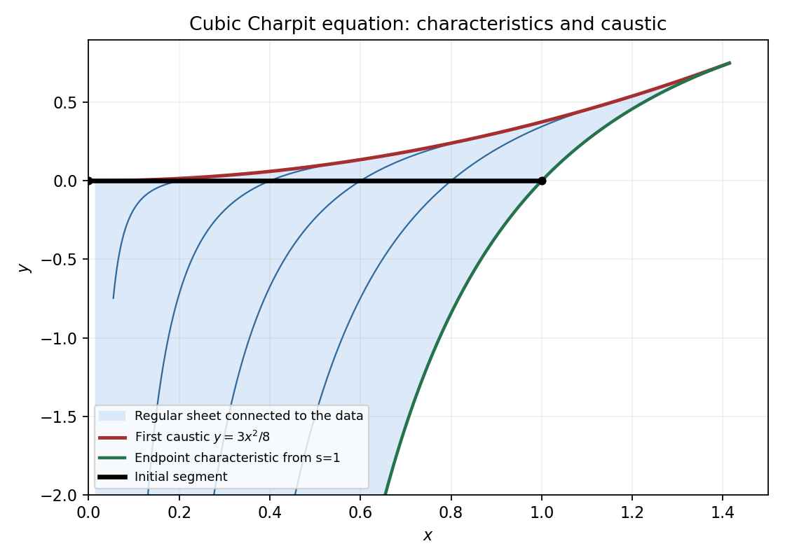
The regular characteristic sheet issued from the initial segment, its endpoint characteristic and the first caustic
. Details. 
In vector form the system is , withFor , its two real distinct eigenvalues are , with left eigenvectors . Thus the system is strictly hyperbolic there; at the eigenvalues coincide and the matrix is defective, so strict hyperbolicity fails. The characteristic directions are .
If , multiplication of by the left eigenvector gives . Since , defineThenConsequently is constant on the minus characteristic curves, and is constant on the plus characteristic curves. One reconstructs , with the essential physical constraint .
For the data on , the nonnegative square root givesThus, on any regular patch, use the two footpoints determined byand put , , selecting branches continuous from the initial point. These implicit algebraic formulas determine the local answer wherever both characteristic curve projections are regular and .
For example, near an initial point with , they give , , so . On an initial interval , define . One instead has andnear the chosen initial point . The radicands must be positive, the footpoints must stay in their indicated initial intervals, and must hold.
There is no continuously differentiable solution realizing the first data set on the entire stated initial line. At , , , and . The minus left eigenvector is and its eigenvalue is zero. The differential equation there would require , but its two sides are respectively and . This is an explicit compatibility contradiction, not merely a loss of a preferred formula. Also, the proposed simple expression independent of does not solve the equation for , because then but .
For the second data set, treat as the evolution variable and let label the initial coordinate. Then and . In the positive quadrant the minus characteristic curves give . The plus characteristic curves satisfy and . Therefore their continuous characteristic curve continuation isAbove the parabola the footpoint is ; below it the plus footpoint is . Each branch directly satisfies both equations and . They agree continuously on , but their derivatives are and , respectively. Thus the continuation is piecewise classical and not continuously differentiable across the parabola. The source's globally continuously differentiable formulation needs this qualification. If only positive initial is intended, the upper rational formula is a classical continuation throughout the positive quadrant, but the region requires incoming information from and is not determined by that positive half of the initial line alone. This illustrates loss of differentiability from square-root hyperbolic source data.
Set and . Balancing , diffusion and the cubic gives , hence . The drift term cancels the contribution in , leavingMultiply by and integrate. The limiting equilibrium has , fixing the constant and giving . The increasing branch from zero to one obeys . ThereforeThe first integral also shows why another turning branch cannot reach the required limit from zero.
At a space-time interior maximum, and . The equation would then give , so . Hence a positive interior maximum is impossible. In particular, a global maximum cannot be attained at an interior point, since the far-field boundary has positive values. If “maximum” instead means every local maximum of an arbitrary signed solution, the calculation only excludes positive local maxima; nonnegativity must be added for the broader usual interpretation. Positive boundary values alone do not impose nonnegativity on arbitrary initial data.
For uniqueness in the standard bounded classical solution class on finite time strips, set , , and . The equation becomeswith , and prescribed . For two solutions let . ThenThe bracket is at most since . Thus solves with , zero initial data and zero boundary difference.
For completeness on the unbounded interval, compare with on a large rectangle. This is a strict positive supersolution becauseFinite-strip boundedness lets its right boundary dominate when the rectangle is sufficiently wide. The weak parabolic maximum principle then bounds by this barrier. Send the width to infinity and then to zero. Hence , giving . The boundedness or a suitable uniform far-field/growth condition is the usual hypothesis that makes this unbounded-domain argument valid; pointwise limits at spatial infinity should not silently replace it. This is similarity reduction for a cubic absorption equation with dilating drift.
Choose the positive Green function conventionAway from its pole, is harmonic, and the maximum principle for harmonic functions makes it positive inside . The sign of its logarithmic singularity is important: it is the convention for , whereas a Green function for has the opposite sign.
Green's second identity, justified by removing a small disk about the pole and taking its radius to zero, givesSince , and vanishes on the outer boundary, this rearranges toThe local logarithmic singularity is integrable, so continuous gives a well-defined volume integral.
In complex coordinates , for the unit disk, useThe numerator has no zeros inside the disk, so its logarithm is harmonic there. On , the numerator and denominator have equal modulus, giving the required zero boundary value. Differentiating in the outward radial direction at givesWith zero forcing the representation therefore becomes the Poisson integralFinally replace by and change variable . Cosine stays the same, sine changes sign and the assumed boundary symmetry leaves unchanged. The integral is therefore invariant, so . Equivalently, reflection produces a harmonic function with the same Dirichlet data, and uniqueness identifies it with the original solution.
Articles by others on the same topic
There are currently no matching articles.