Original solutions to the paper released at the source request. The complete editable transcription is retained in the private examination archive.
Use dimensionless variables , , , , withSubstitution gives the requested system, with dots now meaning differentiation with respect to , andIn particular the same scale for makes the first two coefficients of the cubic equal in magnitude.
Its derivative is . For its two simple zeros areThe cubic increases below , decreases between the two fold points of a critical manifold, and increases above . It has a local maximum at and a local minimum at .
After a rapidly decaying transient response, when its relaxation is faster than the other variables. The reduced autonomous system isFor , the fast dynamics at fixed attracts to the branches where and repels from the middle branch. On the low branch , increases slowly. At its fold point of a critical manifold , the attracting low branch disappears and jumps upward, with nearly constant , to the high branch. On that branch , decreases slowly. At it jumps back to the low branch. These slow arcs and fast jumps form the singular relaxation cycle. For small positive , and parameters bounded away from the fold point of a critical manifold-endpoint cases, the nearby attracting periodic motion has the same pattern. The equilibrium is on the repelling branch: its Jacobian matrix has determinant and trace .
The limiting landing values are after the upward jump and after the downward jump, obtained from the third root of . Thus the two vertical segments in the phase plane plot really connect roots of the same fast equation.
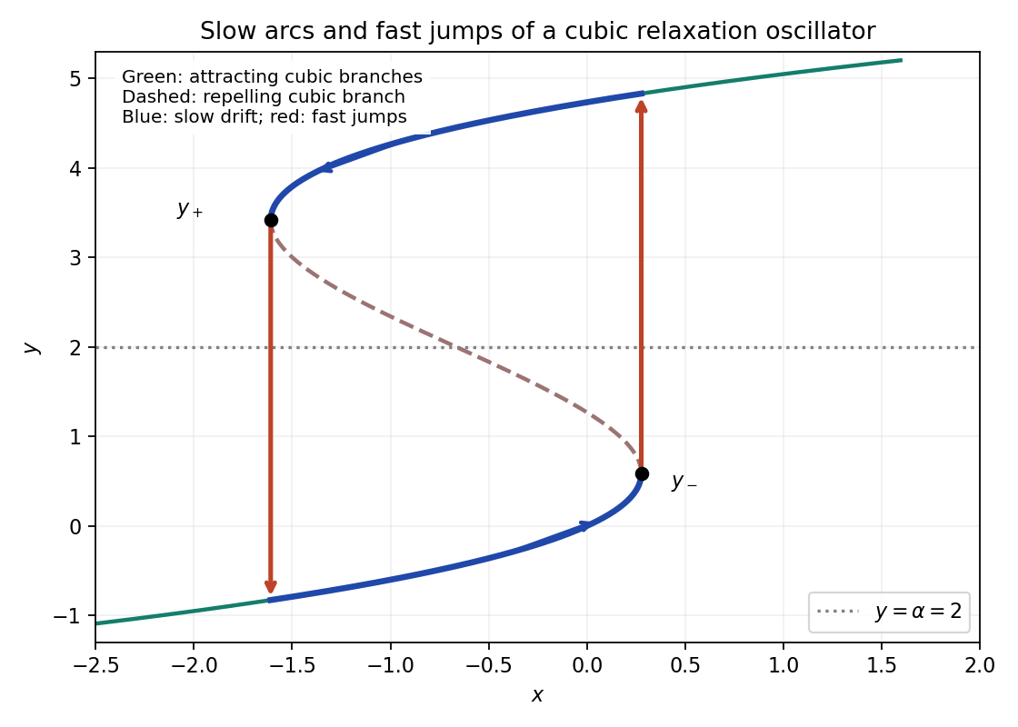
Cubic folds and the singular relaxation cycle: slow drift on attracting branches and fast jumps at nearly fixed x
. Details. 
If , is strictly positive everywhere, so the cubic is monotone and has no fold points of a critical manifold. The reduced equilibrium is asymptotically stable. In factThe only invariant trajectory in the zero-derivative set is the equilibrium, so bounded reduced solutions converge to it; relaxation oscillations disappear.
The stronger condition matters during a fast jump: then varies on the time scale, not on the slow unit scale. Only if adjusts faster still may one keep through that jump. Merely imposing would not justify this reduction on all pieces of the cycle. This is a three-time-scale cubic relaxation oscillator.
For zero damping the conserved mechanical energy isFor , the potential grows to infinity in both directions, so every nonstationary finite-energy trajectory is trapped between two turning points and is periodic; the zero-energy solution is stationary. The case is the harmonic oscillator. The negative- comparison extends the parameter range initially stated in the source.
For , the origin lies in a local potential well, with barriers at of height . A trajectory launched from the origin oscillates precisely when its initial energy is below that barrier:At equality the trajectory approaches a barrier equilibrium asymptotically, rather than being periodic; for example the positive branch is . Above the barrier the trajectory escapes the well. The source's inequality without the absolute value tacitly takes ; for signed initial velocity the energy criterion requires .
Next set and assume . The energy satisfies . This bounds the complete trajectory. The zero-dissipation set is the union of and , and its only invariant trajectory is the origin: a nonzero point on either axis immediately leaves it under the differential equation. The LaSalle invariance principle therefore gives . If as well, damping is absent and that conclusion fails for nonzero ; the positive order-one damping assumption is essential.
For the weakly nonlinear periodic motion, write , set , , and expand . The first correction obeysResonant forcing at the fundamental frequency would generate secular terms. Eliminating both coefficients yieldsConsequently the maximum displacement is for fixed positive . A possible third-harmonic correction is , up to homogeneous amplitude and phase choices. The leading amplitude also balances averaged damping: its slow evolution is , whose nonzero fixed point is attracting. The case is a degenerate zero-amplitude limit, rather than a nonzero limit cycle.
For the singular-endpoint equation, take , , . The indicial equation is . The constant branch violates the zero endpoint value unless its coefficient vanishes; the nontrivial admissible branch therefore has . More precisely, an eigenfunction has and near zero.
Integrate the self-adjoint equation after multiplying by , initially on with :At zero the boundary expression is , the first integrand is , and the second is . Both integrals converge and the boundary term vanishes. Division by the positive weighted norm gives .
The change of coordinate , gives exactlyThus and . To prove a minimum over trial functions, rather than just identify the least eigenvalue, transform the quotient itself:The Dirichlet Poincaré inequality gives the last step, with equality precisely for a nonzero multiple of . The trial class is the nonzero finite-energy class with zero Sobolev traces; endpoint values alone without an integrability requirement do not define a finite quotient. This is the Power-coordinate reduction of a singular Sturm-Liouville quotient.
With diffusion absent, the characteristic equations for a first-order quasilinear equation are , . A characteristic curve labelled by its starting point isThis determines a smooth single-valued solution while is one-to-one. Its derivative isAll characteristic curves move right because . Because , increasing portions of the initial profile have slower characteristic curves ahead than behind, so they steepen. The first positive gradient catastrophe occurs atThis is a minimum when attained. The numerator at such a point is positive and the denominator decreases to zero from above, so .
Resolve the thin transition with and . The leading balance is , where . Integrating once and matching to the state behind givesMatching the state ahead requires and gives the Rankine-Hugoniot speedThe strictly concave graph of has zeros at the two states and lies above its chord, hence is strictly positive between them. Since , through the layer. A heteroclinic profile increasing with can therefore connect the rear state at to the front state at only when . The concavity also gives : characteristic curves enter the viscous shock from both sides. Reversing the states would demand a decreasing profile, contradicting the sign of .
Write the parameter along a characteristic curve as . Charpit's equations areAt , prescribe , , and choose satisfying both and the compatibility relation . Direct differentiation givesThus the initial constraint propagates. A chosen initial-gradient branch is locally unique whenThis is simultaneously the implicit-function determinant for the initial gradients and the projection map determinant for the surface generated by the method of characteristics. Uniqueness continues while that projection map is invertible, the flow remains regular, and distinct characteristic curves do not give competing values at the same point. Multiple initial-gradient branches, characteristic curve initial points or a caustic require separate analysis.
Here the initial coordinate is , so and the equation forces , hence . The projection map determinant on the initial line is , nonzero for . Solving the characteristic curve ordinary differential equations giveswith and . These satisfy both the equation and all the noncharacteristic initial values.
The projection map determinant is . Starting from , the first caustic occurs at . At the initial endpoint the non-characteristic condition fails, and its entire characteristic curve remains the single point ; it does not generate an open region of determination.
The maximal regular sheet connected to the initial line uses . Its interior image is exactlyIndeed the inverse on this sheet isand the inequalities say and . The upper boundary is the caustic; the lower boundary is the characteristic curve from . Endpoints of that latter boundary can be retained as one-sided data. For forward characteristic curves alone, also impose : this retains , with lower boundary zero for and the displayed endpoint characteristic curve for . The other square-root branch belongs to the folded sheet after the caustic and does not provide a unique regular continuation from the initial data.
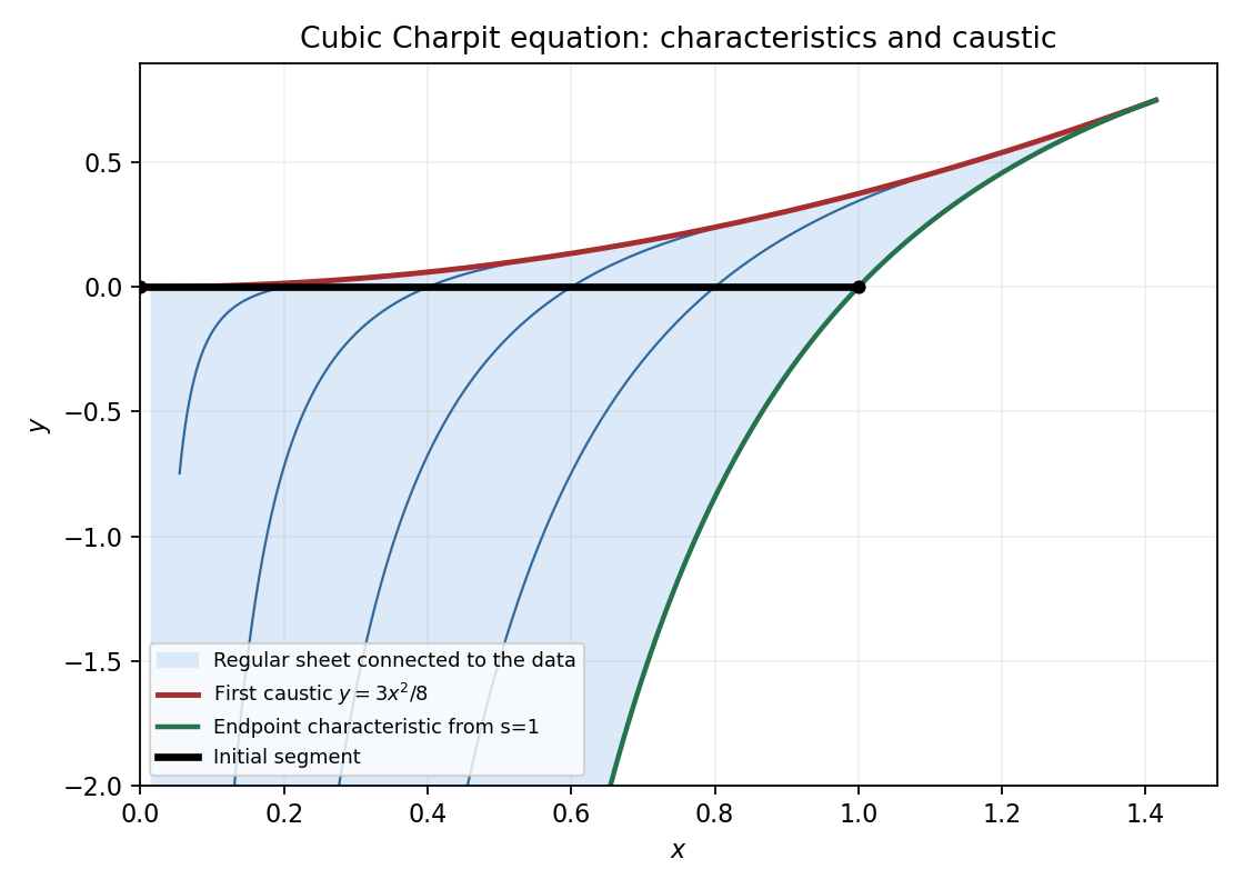
The regular characteristic sheet issued from the initial segment, its endpoint characteristic and the first caustic
. Details. 
In vector form the system is , withFor , its two real distinct eigenvalues are , with left eigenvectors . Thus the system is strictly hyperbolic there; at the eigenvalues coincide and the matrix is defective, so strict hyperbolicity fails. The characteristic directions are .
If , multiplication of by the left eigenvector gives . Since , defineThenConsequently is constant on the minus characteristic curves, and is constant on the plus characteristic curves. One reconstructs , with the essential physical constraint .
For the data on , the nonnegative square root givesThus, on any regular patch, use the two footpoints determined byand put , , selecting branches continuous from the initial point. These implicit algebraic formulas determine the local answer wherever both characteristic curve projections are regular and .
For example, near an initial point with , they give , , so . On an initial interval , define . One instead has andnear the chosen initial point . The radicands must be positive, the footpoints must stay in their indicated initial intervals, and must hold.
There is no continuously differentiable solution realizing the first data set on the entire stated initial line. At , , , and . The minus left eigenvector is and its eigenvalue is zero. The differential equation there would require , but its two sides are respectively and . This is an explicit compatibility contradiction, not merely a loss of a preferred formula. Also, the proposed simple expression independent of does not solve the equation for , because then but .
For the second data set, treat as the evolution variable and let label the initial coordinate. Then and . In the positive quadrant the minus characteristic curves give . The plus characteristic curves satisfy and . Therefore their continuous characteristic curve continuation isAbove the parabola the footpoint is ; below it the plus footpoint is . Each branch directly satisfies both equations and . They agree continuously on , but their derivatives are and , respectively. Thus the continuation is piecewise classical and not continuously differentiable across the parabola. The source's globally continuously differentiable formulation needs this qualification. If only positive initial is intended, the upper rational formula is a classical continuation throughout the positive quadrant, but the region requires incoming information from and is not determined by that positive half of the initial line alone. This illustrates loss of differentiability from square-root hyperbolic source data.
Set and . Balancing , diffusion and the cubic gives , hence . The drift term cancels the contribution in , leavingMultiply by and integrate. The limiting equilibrium has , fixing the constant and giving . The increasing branch from zero to one obeys . ThereforeThe first integral also shows why another turning branch cannot reach the required limit from zero.
At a space-time interior maximum, and . The equation would then give , so . Hence a positive interior maximum is impossible. In particular, a global maximum cannot be attained at an interior point, since the far-field boundary has positive values. If “maximum” instead means every local maximum of an arbitrary signed solution, the calculation only excludes positive local maxima; nonnegativity must be added for the broader usual interpretation. Positive boundary values alone do not impose nonnegativity on arbitrary initial data.
For uniqueness in the standard bounded classical solution class on finite time strips, set , , and . The equation becomeswith , and prescribed . For two solutions let . ThenThe bracket is at most since . Thus solves with , zero initial data and zero boundary difference.
For completeness on the unbounded interval, compare with on a large rectangle. This is a strict positive supersolution becauseFinite-strip boundedness lets its right boundary dominate when the rectangle is sufficiently wide. The weak parabolic maximum principle then bounds by this barrier. Send the width to infinity and then to zero. Hence , giving . The boundedness or a suitable uniform far-field/growth condition is the usual hypothesis that makes this unbounded-domain argument valid; pointwise limits at spatial infinity should not silently replace it. This is similarity reduction for a cubic absorption equation with dilating drift.
Choose the positive Green function conventionAway from its pole, is harmonic, and the maximum principle for harmonic functions makes it positive inside . The sign of its logarithmic singularity is important: it is the convention for , whereas a Green function for has the opposite sign.
Green's second identity, justified by removing a small disk about the pole and taking its radius to zero, givesSince , and vanishes on the outer boundary, this rearranges toThe local logarithmic singularity is integrable, so continuous gives a well-defined volume integral.
In complex coordinates , for the unit disk, useThe numerator has no zeros inside the disk, so its logarithm is harmonic there. On , the numerator and denominator have equal modulus, giving the required zero boundary value. Differentiating in the outward radial direction at givesWith zero forcing the representation therefore becomes the Poisson integralFinally replace by and change variable . Cosine stays the same, sine changes sign and the assumed boundary symmetry leaves unchanged. The integral is therefore invariant, so . Equivalently, reflection produces a harmonic function with the same Dirichlet data, and uniqueness identifies it with the original solution.
Articles by others on the same topic
There are currently no matching articles.