For the general equation the Charpit's equations areAt parameter time zero set and choose to satisfy and . The chain rule givesso remains zero. The non-characteristic condition is , ensuring a local graph.
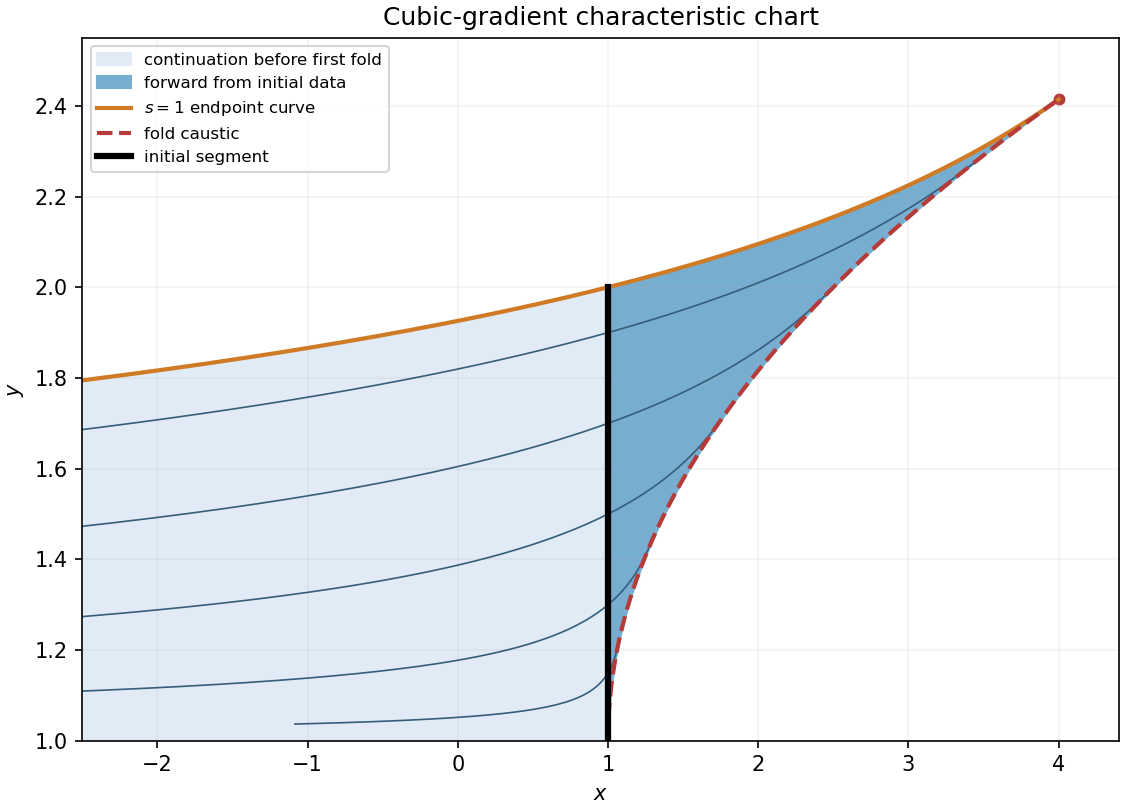
For the particular equation put and label the initial curve by , , , . Compatibility gives and , hence the unique real choice . Integrating the characteristic equations givesThe projection determinant is . Initially ; its first zero is . At that fold,To describe the entire chart attached to the data before the fold, put and . Elimination gives andThe initial-endpoint constraint therefore gives the uniquely determined chartThe boundary is included as inherited endpoint data; open-domain statements use strict inequality there. The fold is excluded. For forward characteristic times only, , impose additionally . The source excludes , so is not a non-characteristic initial point. The sheet beyond the fold does not extend this initial graph uniquely.

The coefficient matrix of is . Its distinct eigenvalues are for every , so the system is strictly hyperbolic. Define . Thenthe derivative terms cancel, as do the sources . Hence is constant on the plus-family characteristics.
The data give , so throughout their domain of dependence . The minus-family speed is then : the other characteristics are the horizontal lines . Substitution into the second PDE, or its minus-characteristic compatibility relation, gives . Integrate at fixed using and retain the positive branch:Indeed , , , so ; similarly .
For the lower edge of the region determined solely by the given data is the plus characteristic from . Write it , where the exact boundary characterization isThe determined region is , with strict inequality for its interior. Both backward characteristic families there reach the supplied initial half-line. Below this boundary a backward plus characteristic would require initial data below , which were not supplied; extending the displayed formulas there gives a possible continuation but is not forced by the data. An elementary expression for is unnecessary: its initial-value ODE defines it uniquely and the requested other family already has the explicit form . The sketch integrates only this boundary for illustration.
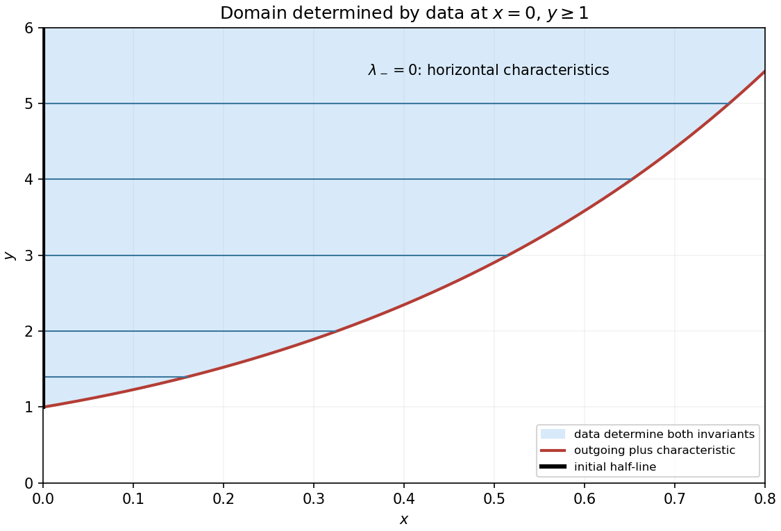
Horizontal minus characteristics and the outgoing plus boundary of the determined region
. Details. 
At such an interior backward-in-time maximum, spatial differentiation gives and . Comparison with earlier times at the same spatial point gives the one-sided time derivative ; differentiability makes this the usual derivative. Consequently , contradicting the strictly positive source . Therefore no such maximum can occur. The temporal one-sided argument matters because the condition concerns only the past of the candidate point.
The stated pointwise boundary limits do not imply uniqueness. A counterexample to homogeneous uniqueness isIt is smooth for . Writing , differentiation givesFor fixed positive , as and as ; for fixed positive , it also tends to zero as . Thus if is one solution, satisfies the same equation and every printed boundary limit for any constant . Part (d) supplies such a particular solution, so this is a genuine family of distinct solutions, not merely a formal obstruction.
This is corner-source nonuniqueness for a degenerate parabolic problem. The peak diverges towards the missing corner ; pointwise initial limits at each fixed do not exclude it. The preceding maximum argument fails to force uniqueness because a supremum over an entire past strip need not be attained or finite.
A customary bounded-solution condition restores the intended result. If the difference of two solutions is bounded on every finite time strip, subtract . Its operator equals , excluding a positive past maximum; the linear barrier controls spatial infinity, and the homogeneous initial/boundary values control the parabolic boundary. Letting gives ; applying the same argument to gives . This proves uniqueness in that additional bounded class, which the printed pointwise limits alone do not specify.
Choose the positive causal sign convention , so the forced equation is . With source , a forward Green's function satisfiesIt vanishes at , decays at spatial infinity in the chosen bounded evolution class, and has the temporal jump . Away from the source it solves the homogeneous equation. Equivalently one may reverse both the Green-function operator and its source sign to use the original printed operator.
To select the physical zero-initial-data solution one also excludes extra corner-source terms of the kind found in (b). With this causal bounded convention the solution representation isA mere pointwise statement of the three boundary limits does not by itself provide that uniqueness convention.
The forcing contains , so matching it with a single similarity variable requires . For , , substitution givesMatching the source selects and gives . Multiplying the first-order equation for by yields , so . The limits at zero and infinity give , . HenceFor fixed positive , the initial limit is also zero because the exponential dominates . The function decreases to at and increases thereafter. ThereforeThe axis limits are zero, but there is no joint limit at : approaching along gives . This does not violate any of the printed fixed-variable limits. It is this bounded similarity solution whose minimum was calculated; the unbounded corner-source additions in (b) need not have the same minimum.
Articles by others on the same topic
There are currently no matching articles.