Original solutions to the paper released at the source request. The complete editable transcription is retained in the private examination archive.
Define the auxiliary variable . Differentiating gives , while rearrangement gives . Conversely eliminating recovers the second-order equation, so this phase plane system is equivalent. At an equilibrium forces , and the first equation then forces . Its Jacobian matrix isThus . Expanding givesFor sufficiently small positive both are positive: the equilibrium is an unstable node. For negative the fast root is negative and the slow root positive, so it becomes a saddle equilibrium.
The nullcline is . Write . Away from it at an order-one distance, is order one on the indicated finite phase-space scales. Thus while : the trajectory changes on the fast time in a singular perturbation , with only an change in . Equivalently , which explains the nearly horizontal motion.
For positive , makes the branches fast attracting and the middle branch fast repelling. The arrows point right where and left where , carrying a generic off-nullcline point towards an attracting branch. The reduced description changes near a fold, where ; the rapid/slow distinction there needs a separate transition layer.
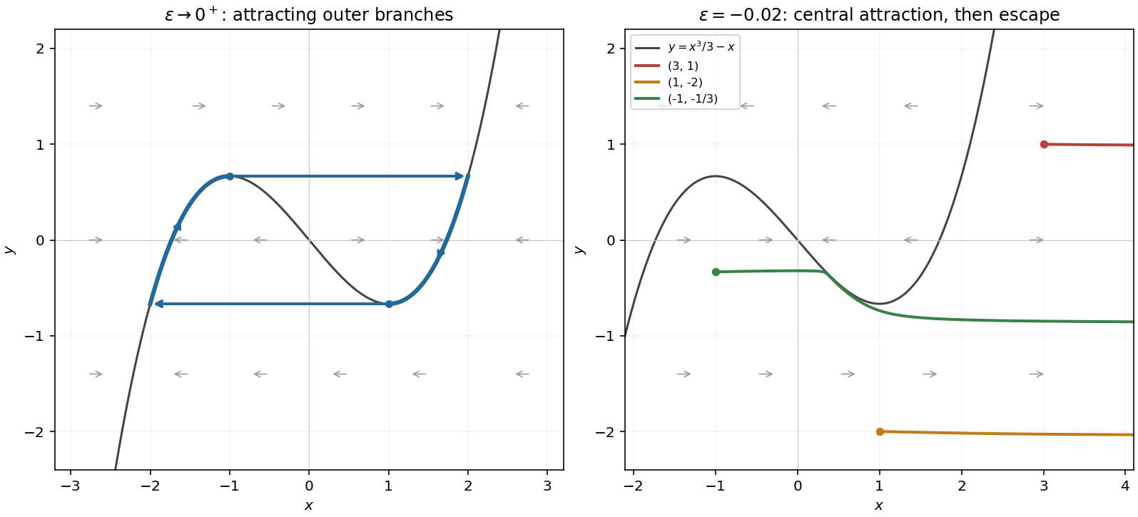
The left panel shows positive ; the right panel shows negative , including the three specified starting points. Horizontal arrows indicate the leading fast motion.
On the attracting right branch, and , so the motion goes from towards the fold . At essentially fixed it jumps to the other attracting root . The left branch then carries it to , where it jumps right to . This gives the clockwise limiting relaxation oscillation shown in the preceding figure.
Along a slow branch , differentiation gives . The right-branch time isReflection symmetry gives the same time on the left. The fast jumps take a time tending to zero as , as do the fold-transition corrections at leading order. HenceThis is a leading asymptotic period, not an exact finite- equality.
For negative the fast arrows reverse: the outer branches become repelling and the middle branch attracting. On the middle branch the slow equation is , so the slow motion goes away from the saddle equilibrium at zero towards a fold.
At , , so : the trajectory immediately escapes to the right. At , , so it also moves rapidly right and escapes. In each case the large- balance is , with decreasing; it is not a bounded relaxation cycle.
At , , so the initial fast motion is rightward. At nearly fixed it approaches the attracting middle root of , approximately . It then moves slowly down/right along the middle branch towards , leaves that fold to the right, and eventually escapes. These are the small-negative- limiting descriptions; the fold locations and fast landing point receive small corrections. The right panel of the figure distinguishes this slow excursion from the two immediate escapes.
Put . Then and the endpoint conditions become . The transformed eigenvalue equation is , soZero and negative yield no nonzero solution with both endpoint values zero.
For the usual unweighted inner product, the operator is not self-adjoint: its formal adjoint is . The mismatch is already visible on compactly supported test functions, so endpoint conditions cannot remove it. With the different weight one does obtain a symmetric Sturm-Liouville form, since . Thus the inner-product convention matters; the real spectrum alone does not prove self-adjointness in the unweighted space.
Use the complex inner product , linear in its second argument. Exchanging the order of integration givesSince the kernel is real, the adjoint operator is thereforeor, renaming variables, . Continuity of the kernel on the compact integration square justifies these integrals and the exchange.
Symmetry makes the adjoint kernel equal to the original kernel, so . For a nonzero eigenfunction ,Thus . The argument includes the zero eigenvalue and does not require normalizing the eigenfunction.
Antisymmetry instead gives , so is skew-adjoint. Its quadratic form satisfies . Hence an eigenpair satisfiesNonzero eigenvalues are purely imaginary in the complexified function space; zero is allowed as well. On a strictly real vector space this means there are no nonzero real eigenvalues.
Write . The separated kernel givesThus its image is . Since and , its matrix on this basis is . ThereforeBoth eigenspaces have dimension one, and there are no further nonzero eigenvalues because every such eigenfunction belongs to the image. The zero eigenspace is , which is infinite-dimensional. One explicit nonzero example is , orthogonal to both and .
The image of consists only of . If were such a function, its endpoint values would give and its midpoint value , forcing , . That combination is , which differs from , for example at . Continuity makes the same argument valid for equality almost everywhere. Thus the forcing is outside the image and no solution exists.
Here belongs to the image. Matching the two coefficients using gives , . ConsequentlyThere are infinitely many solutions, since any element of the infinite-dimensional kernel may be added.
The eigenvalues of are , and zero, none equal to one. On the map is an invertible two-dimensional operator; on it is . Hence it is invertible on all of . Thus has exactly one solution. This is the finite-rank Fredholm alternative; no range obstruction survives the nonresonant identity term.
The quantity inside a fixed interval changes by influx at its left endpoint minus outflux at its right endpoint:In a smooth region the fundamental theorem of calculus turns this into . Since the interval is arbitrary, the local conservation law is .
For a jump at , write the two smooth pieces using a step function. The singular part of is and that of is . Cancellation gives the Rankine-Hugoniot conditionThe same identity follows by applying conservation to a shrinking moving control interval across the shock.
In smooth regions the characteristic equations are and . If labels the initial point, their parametrization isFor the two constant states, characteristics from the left have speed one and those from the right speed zero; they would overlap. The entropy solution replaces the overlap by a compressive shock. Its speed isThusThe left parametrization is retained only for , and the right parametrization only for . The characteristic speeds obey , so characteristics enter the shock from both sides.
Before intersection, the characteristic map is , with derivative . Because the initial profile decreases, higher-density characteristics behind move faster than lower-density characteristics ahead. Compression therefore forms shocks, which absorb more characteristics. The far states remain one and zero, so a shock joining their limiting traces has speed tending to .
The precise large-scale interpretation uses . The rescaled initial transition tends to a step, and entropy comparison for the convex flux givesOne way to see the comparison is to choose distant initial points beyond which the profile is within of each far state. Step profiles with those nearby states bracket it; their shock speeds tend to as , while their fixed initial locations disappear after division by .
A fixed translation of the shock can persist. If the deviation from a reference step is integrable, its signed mass fixes a phase shift. Without such a tail assumption one should assert convergence on the scale and , rather than claim that the exact line is the unshifted asymptote for every smooth initial transition.
Mass preservation of a nonnegative finite-mass profile requires . Balancing and requires . ThereforeThe similarity ODE isFor a source-type profile adjoining vacuum, the integration constant is zero. The positive branch is for positive , terminated by a shock into zero. Normalize the mass:Thus a unit-mass similarity solution isAt the moving right edge, equals , so the Rankine-Hugoniot condition is satisfied. The characteristic speeds satisfy , making it an entropy shock. The left edge meets vacuum continuously. As the mass concentrates at the origin; this is a source solution, not a claim that every finite-mass initial profile equals it at finite time.
For the general equation the Charpit's equations areAt parameter time zero set and choose to satisfy and . The chain rule givesso remains zero. The non-characteristic condition is , ensuring a local graph.
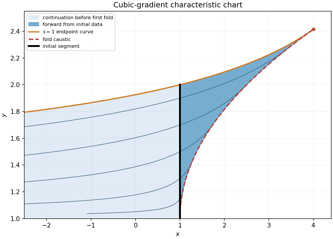
For the particular equation put and label the initial curve by , , , . Compatibility gives and , hence the unique real choice . Integrating the characteristic equations givesThe projection determinant is . Initially ; its first zero is . At that fold,To describe the entire chart attached to the data before the fold, put and . Elimination gives andThe initial-endpoint constraint therefore gives the uniquely determined chartThe boundary is included as inherited endpoint data; open-domain statements use strict inequality there. The fold is excluded. For forward characteristic times only, , impose additionally . The source excludes , so is not a non-characteristic initial point. The sheet beyond the fold does not extend this initial graph uniquely.


The coefficient matrix of is . Its distinct eigenvalues are for every , so the system is strictly hyperbolic. Define . Thenthe derivative terms cancel, as do the sources . Hence is constant on the plus-family characteristics.
The data give , so throughout their domain of dependence . The minus-family speed is then : the other characteristics are the horizontal lines . Substitution into the second PDE, or its minus-characteristic compatibility relation, gives . Integrate at fixed using and retain the positive branch:Indeed , , , so ; similarly .
For the lower edge of the region determined solely by the given data is the plus characteristic from . Write it , where the exact boundary characterization isThe determined region is , with strict inequality for its interior. Both backward characteristic families there reach the supplied initial half-line. Below this boundary a backward plus characteristic would require initial data below , which were not supplied; extending the displayed formulas there gives a possible continuation but is not forced by the data. An elementary expression for is unnecessary: its initial-value ODE defines it uniquely and the requested other family already has the explicit form . The sketch integrates only this boundary for illustration.
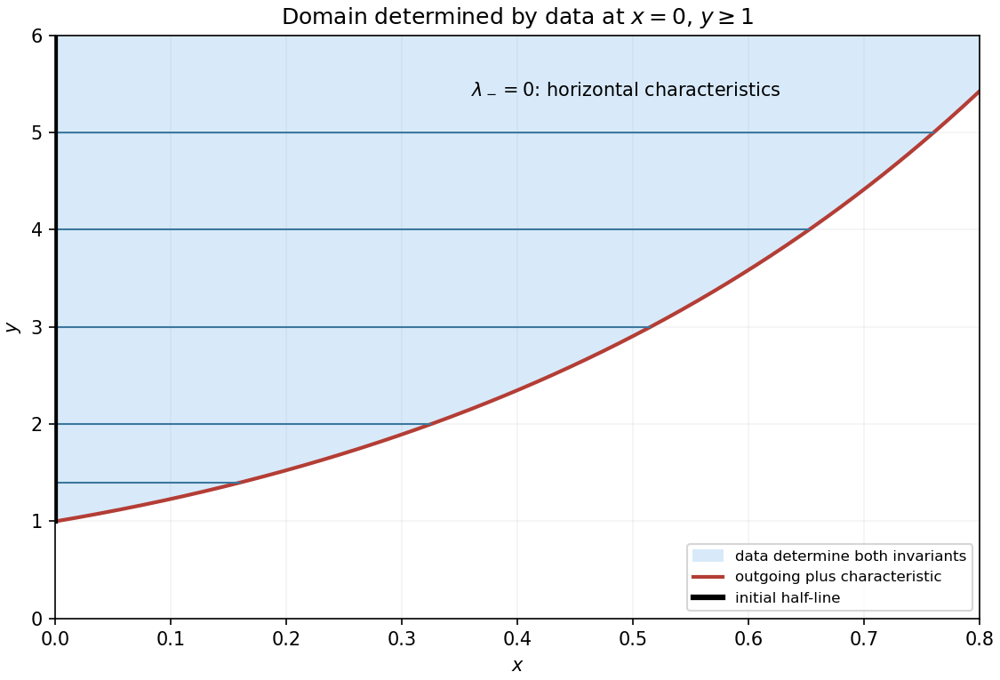
Horizontal minus characteristics and the outgoing plus boundary of the determined region
. Details. 
At such an interior backward-in-time maximum, spatial differentiation gives and . Comparison with earlier times at the same spatial point gives the one-sided time derivative ; differentiability makes this the usual derivative. Consequently , contradicting the strictly positive source . Therefore no such maximum can occur. The temporal one-sided argument matters because the condition concerns only the past of the candidate point.
The stated pointwise boundary limits do not imply uniqueness. A counterexample to homogeneous uniqueness isIt is smooth for . Writing , differentiation givesFor fixed positive , as and as ; for fixed positive , it also tends to zero as . Thus if is one solution, satisfies the same equation and every printed boundary limit for any constant . Part (d) supplies such a particular solution, so this is a genuine family of distinct solutions, not merely a formal obstruction.
This is corner-source nonuniqueness for a degenerate parabolic problem. The peak diverges towards the missing corner ; pointwise initial limits at each fixed do not exclude it. The preceding maximum argument fails to force uniqueness because a supremum over an entire past strip need not be attained or finite.
A customary bounded-solution condition restores the intended result. If the difference of two solutions is bounded on every finite time strip, subtract . Its operator equals , excluding a positive past maximum; the linear barrier controls spatial infinity, and the homogeneous initial/boundary values control the parabolic boundary. Letting gives ; applying the same argument to gives . This proves uniqueness in that additional bounded class, which the printed pointwise limits alone do not specify.
Choose the positive causal sign convention , so the forced equation is . With source , a forward Green's function satisfiesIt vanishes at , decays at spatial infinity in the chosen bounded evolution class, and has the temporal jump . Away from the source it solves the homogeneous equation. Equivalently one may reverse both the Green-function operator and its source sign to use the original printed operator.
To select the physical zero-initial-data solution one also excludes extra corner-source terms of the kind found in (b). With this causal bounded convention the solution representation isA mere pointwise statement of the three boundary limits does not by itself provide that uniqueness convention.
The forcing contains , so matching it with a single similarity variable requires . For , , substitution givesMatching the source selects and gives . Multiplying the first-order equation for by yields , so . The limits at zero and infinity give , . HenceFor fixed positive , the initial limit is also zero because the exponential dominates . The function decreases to at and increases thereafter. ThereforeThe axis limits are zero, but there is no joint limit at : approaching along gives . This does not violate any of the printed fixed-variable limits. It is this bounded similarity solution whose minimum was calculated; the unbounded corner-source additions in (b) need not have the same minimum.
Articles by others on the same topic
There are currently no matching articles.