Past exam of the mathematics and the environment and mathematical physiology course of the University of Oxford / 2010 / A / 3

Resolve gravity into components $g\sin \alpha$ down the bed and $-g\cos \alpha$ normal to it. For slow incompressible flow, inertia is negligible and Cauchy momentum equation reduces to the divergence of the stress tensor plus the gravitational force density being zero. Write the dominant shear component as $\tau ={\sigma }_{xz}$ and the leading normal stresses as $-p$.

The shallow-ice approximation assumes a small thickness-to-length ratio. Vertical variation of the shear is retained in the along-bed equation, while longitudinal deviatoric-stress gradients and the shear contribution to the normal equation are higher order. The leading balances are consequentlyThe second is a hydrostatic pressure balance; the first balances gravitational driving and the surface-induced pressure gradient against vertical shear. This approximation requires shallow geometry and sufficiently slow flow, not a Newtonian constitutive equation for ice.

Measure pressure relative to atmospheric pressure. At leading order the stress-free upper surface gives $p(H)=0$, $\tau (H)=0$. Integrating the normal balance first yieldsAt fixed $z$, $p_x=\rho g\cos \alpha H_x$. Therefore ${\tau }_z=\rho g(\cos \alpha H_x-\sin \alpha )$, independent of $z$. Integrating from $z$ to $H$ givesThis is linear in $z$, is zero at the surface, and reaches its basal value at $z=0$. In particular the surface slope modifies the shear driving; a flat upper surface relative to the horizontal eliminates it in this approximation.

Set $G=\rho g(\sin \alpha -\cos \alpha H_x)$. For downstream shear $G\ge 0$, Glen's flow law and the no-slip boundary condition giveHere $A$ is the ice rate factor, distinct from the cross-sectional area in the river problem. Integrating this velocity profile through the thickness gives the volume flux per unit valley width:The factor $H^{n+2}$ combines the depth-dependent shear stress, integration to obtain velocity, and integration to obtain flux. If reverse shear is admitted for noninteger $n$, the signed version of Glen's flow law is $u_z=A|\tau {|}^{n-1}\tau$; the displayed unsigned power presumes the downstream regime.

A typical net ice accumulation curve decreases downstream: snow gain at high elevation, zero at the equilibrium line, and negative values in the ice ablation zone. In a steady glacier with zero volume flux at its head, $Q(x)={\int }_0^{x}a(X)dX$. If its terminus also has zero volume flux, a natural glacier length $L$ is the positive root of ${\int }_0^{L}a(X)dX=0$, with the integral positive between the endpoints. Such a root requires a suitable given accumulation profile; it is not guaranteed by dimensional analysis alone.

Let $a_0$ be a representative accumulation rate and $K=A(\rho g\sin \alpha {)}^n$. ChooseUsing $x=L\hat{x}$, $H=H_{\ast }\hat{H}$, $Q=Q_{\ast }\hat{Q}$, $t=t_{\ast }\hat{t}$, $a=a_0\hat{a}$, both terms in mass conservation have scale $a_0$. The dimensionless flux isDropping hats gives the required partial differential equation. The parameter measures the surface-thickness slope correction relative to the bed slope. For the linear example $a=1-2x$, accumulation changes sign at $x=1/2$ and its integrated balance vanishes at $x=1$.

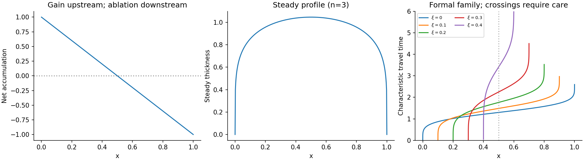
Write $A(x)=x-x^2$, $q=1/(n+2)$ and $p=(n+1)/(n+2)$. Integrating the steady mass conservation equation from the head givesFor the time-dependent first-order equation $H_t+H^{n+1}{H}_x=1-2x$, method of characteristics gives $\dot{x}=H^{n+1}$ and $\dot{H}=1-2x$. Consequently $d[H^{n+2}/(n+2)-A(x)]/dt=0$. On a characteristic starting at $(\xi ,0)$ with zero thickness,On a characteristic emitted by the boundary $x=0$, the invariant is zero and $H=H_0(x)$. The travel time of the one emitted at time zero isThe incomplete beta function is finite at both endpoints because $0<p<1$ for the physical exponents $n>0$. Before characteristic crossings, the initial-data branch and boundary-data branch have the displayed forms in the source, with the appropriate emission time $t-f(x)$ for the latter.

Glacier characteristic admissibility gives a substantive domain restriction. Factoring the invariant gives $A(x)-A(\xi )=(x-\xi )(1-x-\xi )$. A positive forward branch requiresEquivalently it is the image of this parameter domain under $(\xi ,x)\mapsto (x,t(\xi ,x))$, restricted further to regions where that map is single-valued. Characteristics cannot start with positive thickness growth at $\xi >1/2$, where the prescribed initial rate $H_t=1-2\xi$ is negative. This is why the printed piecewise expression is a formal characteristic construction, not a global nonnegative solution from a bare bed. For example for $x>1/2$, putting $L_{\xi }=1-2\xi$ givesBoth factors increase with $\xi$ there, so no positive initial-data branch exists at that $x$ for $0<t<f(x)$, contrary to a literal global reading of the first case. Compression can also make characteristics intersect; entropy solutions then require shock waves.

One can nevertheless give the exact zero-thickness endpoint locus of these formal characteristics. Let $K=f(1)=(n+2{)}^{-p}B(q,q)$. At $x=1-\xi$ the change of variable $z=\xi +(1-2\xi )y$ givesThis is the formal snout locus inferred from the given characteristic family; it retreats from $1$ towards $1/2$. It is not justified as the physical terminus of an accumulating glacier formed from zero initial ice. In particular it says nothing about a positive advancing snout at $t<K$. A physical free boundary problem must specify no ablation on a bare bed, maintain $H\ge 0$, and select an entropy solution or retain the small slope regularization. Those additional conditions are absent from the printed first-order construction. Thus a unique global physical snout trajectory cannot be claimed from that construction alone. The steady endpoint remains $x=1$. The degenerate $n=0$ limit would instead have the same endpoint time $K$ for every initial characteristic, so the inverted formula presumes $n>0$.